
Determining a Zero-point Variation Map for the WFI
The figure below shows the analysis of the observations of standards in all chips of the WFI. The data was bias subtracted and flat-fielded using twilight sky flats. Aperture photometry was carried out on the reduced frames using a “diaphragm” diameter of 11 arcsec. The atmospheric extinction coefficients were determined using observations of the RU149 Landolt field at 3 different airmasses. Then, the aperture magnitudes were corrected to the extra-atmospheric values. The top-left panel shows the color-color diagram of the stars used in the color-equation determination (large blue dots), together with the locus for normal galactic dwarfs from Schmidt-Kaler (1982), and the locus of the synthetic Kurucz models for dwarfs (black line), and super-giants (red line).
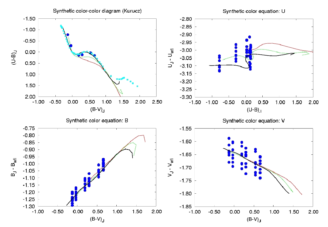
The upper-left, lower-left, and lower right diagrams show the observed color equations for U, B, and V respectively. Also plotted are the synthetic color equations. The large spread in zero-point, approximately 10% peak-to-valley, is apparent in this figure.
We have designed a method to derive a zero-point correction map using three simple dithered exposures. You can find the details of the method in this document (Selman 2003). The same field of stars is imaged in rapid succession with the second image offset a small amount in the north-south direction, and the third image offset a small amount in the east-west direction. Aperture photometry is carried out for the same list of stars in all three images. If there is not zp variations, then the same stars would have the same magnitudes in all three chips (apart from a possible common change in atmospheric transparency). The zp variations induce systematic magnitude differences. These are modeled using a two dimensional Chebyshev basis, shown in the figure below.
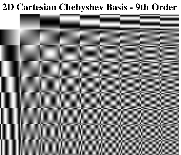
In this figure each small square represents the whole WFI field of view. With a least-squares procedures we determine the 91 coefficients that best represents the magnitude-difference data. The resultant zero-point correction map is shown in the figure below.
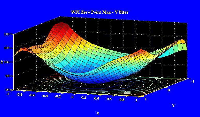
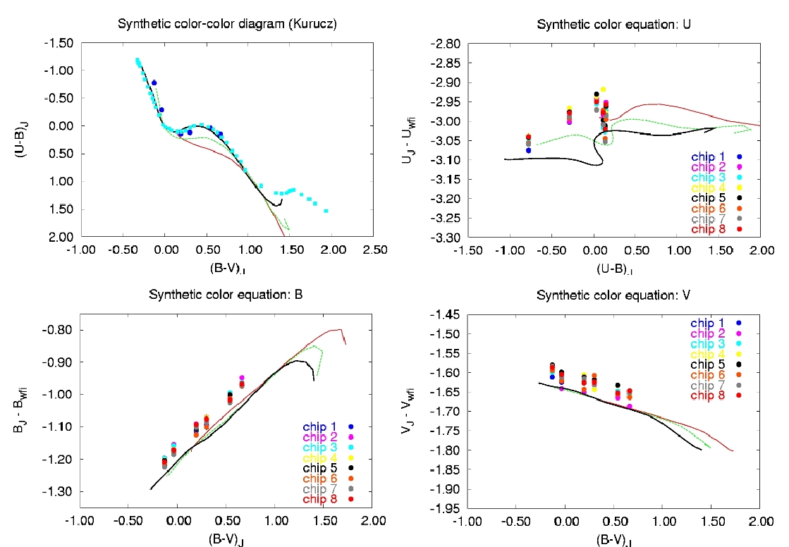
In this figure the z axis shows the percentile variation from a fiducial point on the mosaic. The sense of the correction is that the measured magnitudes of the stars near the center of the mosaic needs to be made more negative, that is, they should be brightened. After applying the above zero-point map to the RU149 data presented above, we reduce the scatter from 0.034 to 0.009 in V, from 0.029 to 0.010 in B, and from 0.040 to 0.014 in U. Notice that we have used the same mask, the one determined for the V filter, on all filters. The figure below shows the reduction on the scatter graphically.
The above correction map can be found in the file:
Vfinal_Cheb9.coefs |
which contains the coefficients of a 9th order cartesian 2D polynomial approximating the zero-point variation map.
The method is still experimental, and the above zero-point map should be used with caution, that is, the data corrected with such a correction map should be validated with independent observations of Landolt field with stars scattered across the mosaic (such as Landolt SA98) to determine the reduction in the scatter in your data. Observations of such a field are done as part of the standard calibration plan.
The following programs have been used in the production of the above zero-point correction maps. I place the source code here for completeness, as is. The software is not yet supported in any manner neither by ESO nor by its author. Perhaps in the future, after further testing, a user friendly version will be made available.
DESCRIPTION |
SCRIPT |
|---|---|
Python library containing routines to interface with IRAF scripts, and the ds9 image display program. |
|
Python library containing the specific routines needed for the zero-point variation analysis. |
|
Python script used for the aperture photometry in a series of dithered images. This is used to produce the files for zpAnalyze.py |
|
Python scripts that analyses the previous data in terms of Chebyshev polynomials, and produces the zero-point correction map. |
|
Python script used to display the zero-point correction map. |
|
Python script used to correct aperture photometry data. |
zpCorrect.py |
>Set of IRAF wrapper scripts to be called from the command line. shiraf stands for shell-iraf. These routines are called from the python scripts. |