
MATISSE p2 tutorial
1: Phase 2
The Phase 2 process begins when you have been awarded observing time and received an email from the ESO Observing Programmes Office (OPO) announcing that the allocation of time for the coming period has been finalized. The detailed information about how much time was awarded and other relevant details (the "Web Letter") can be viewed by logging into your UserPortal account and clicking on "Check the time allocation information" under the Phase 1 header.
Let's assume you were granted observing time with MATISSE in service mode. This means that you have to prepare your Phase 2 material including observation blocks, instructions (ReadMe), and finding charts with the p2 web interface before a deadline given in the Web Letter (link). We recommend you collect all the necessary documentation first:
- The MATISSE User Manual
- The MATISSE Template Manual
- The VLTI User Manual
- The VLT Service Mode Guidelines
This tutorial provides a step-by-step example of the preparation of a set of OBs for MATISSE, the mid-infrared 4-telescope beam combiner for the VLTI. Observing preparation for all telescopes on Paranal, including the VLTI, must use the new p2 web interface. Please see http://www.eso.org/sci/observing/phase2/p2intro.html for more information on how to use p2.
2: Goal of the tutorial
In this tutorial we will prepare a concatenation of a science target (SCI) OB and one or two OBs (CAL) for the calibrator that performs observations in the L and N bands at low spectral resolution. Typically, MATISSE service mode observations use this type of OB container, with either a CAL-SCI-CAL OB sequence (e.g., for separate LM and N-band calibrators), or a CAL-SCI or SCI-CAL sequence. For narrow-field off-axis observations with GRA4MAT, only a SCI OB is required.
Please note that when creating concatenations for an imaging run (type of observation, as defined in the acquisition template), these must be created within a single group container (including OBs for all requested/approved VLTI configurations). Please see the Imaging Tutorial for detailed instructions.
The sample OBs will illustrate the use of a variety of features of p2 and illustrate the kind of decisions to be taken at the time of preparing in advance an observing run, as well as some aspects that are specific to the preparation of OBs for VLTI and MATISSE.

3: Creating an OB container and defining OBs
This tutorial was created using the p2demo account at http://www.eso.org/p2demo. You can use this account as a sandbox for learning how to use p2. To create OBs for your own runs, go to http://www.eso.org/p2 and login to your user portal account. You will then see your own runs.
If instead you are using the p2demo account, runs for a number of instruments appear in the folders area on the left, since the same tutorial account is used for all of them. Select the folder named MATISSE (with ID 60.A-9252(N) and click the "+" sign in front of it.
When you select a tutorial run and click the "+" sign, a number of folders may appear that were created by other users. To create new containers and OBs, you should create a new folder first and open it just like you see in the screenshot below. To change the name of the folder, click the name in the window on the right.
3.1: OB definition
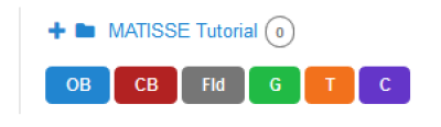
The colored buttons under the folder name allow you to create a new OB, calibration block, folder, group-, time link-, and concatenation containers, in this order. (See here for more information.)
Clicking the button C for a new concatenation, the following window appears. By clicking the name of the concatenation in the window on the right we have already changed it to "Arcturus", the target we will observe. All MATISSE OBs (except in visitor mode!) must be part of concatenations, which is a type of container in which OBs are executed in sequence.
Please note that we have also clicked the "+" sign that was displayed next to the concatenation after it was created to display the blue OB and red CB buttons.
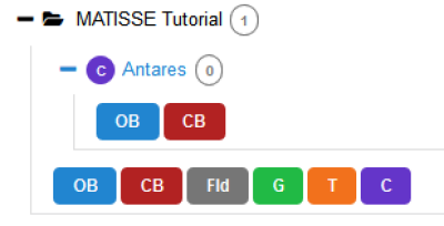
For MATISSE, the allowed sequences are CAL-SCI and CAL-SCI-CAL. To add OBs to a concatenation, we click the blue-colored OB button directly under the concatenation name above. Please give the OBs names beginning with either "CAL_" or "SCI_". We start with the definition of the calibrator observation. To select for each science target a calibration target, ESO offers the CalVin tool. CalVin selects suitable calibrators based on different user criteria. Ideally you would wish to have a calibrator star as close as possible to and of similar brightness as your science target.
3.1.1 Target information
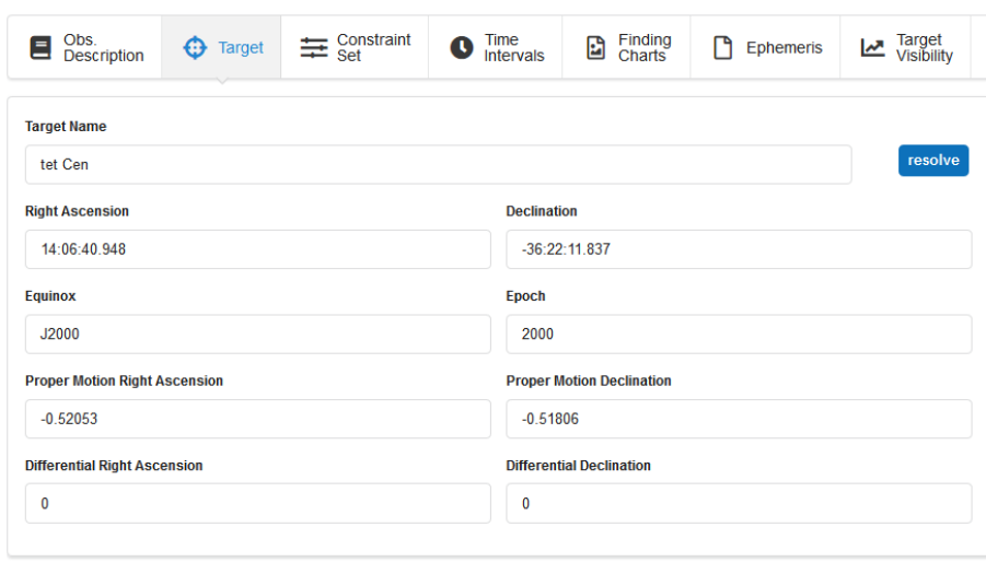
In the window below, we selected the target tab which allows to enter a target by name and resolves it automatically. We already entered the name of our target and resolved it. Please note: you must remove the spaces from the target name after resolving with Simbad!
We will add/modify information related to the OB first in each of the tabs displayed in the row right under the header line.
3.1.2: Constraint Set
All service mode runs need to have a set of constraints which indicate under which conditions OBs can be executed. You can do this by clicking on the Constraint Set icon.
Name:
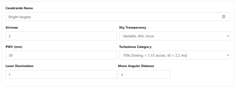
First, give a descriptive name to the constraint set about to be defined. Here, we want to define a constraint set for a bright target, so we call it "Bright". A constraint set can be copied to other runs by using "Copy Constraint Set" under the "Edit" drop-down menu near the top of p2.
Sky transparency:
The MATISSE instrument webpage lists the conditions that are required for MATISSE observations, depending on the correlated magnitude of the target. In our case, the required Sky Transparency condition is "Variable, thin cirrus" for a bright target.
Seeing:
Like for the Sky Transparency, the MATISSE instrument webpage tells us that, given the L-band flux of the target, we require a seeing ≤ 1.15" and τ0 > 2.2 ms, which corresponds to conditions encountered with a 70% chance, i.e, a Turbulence category of 70%. Hence we select the 70% for this category.
Note that in your Phase 1 proposal you already specified some of these constraints (sky transparency and turbulence category) according to the requirements. You must make sure that none of the constraints specified in Phase 2 is more stringent than the corresponding ones specified at Phase 1.
Moon distance:
Should be 3 degrees for guide stars with V < 9, and 5 degrees for V > 9.
Precipitable Water Vapor (PWV):
If using the GRA4MAT setup, the PWV constraint should not be worse than 10 mm.
3.1.3: Time intervals
Several type of time intervals are known to service mode users, two of which are available for VLTI observations.
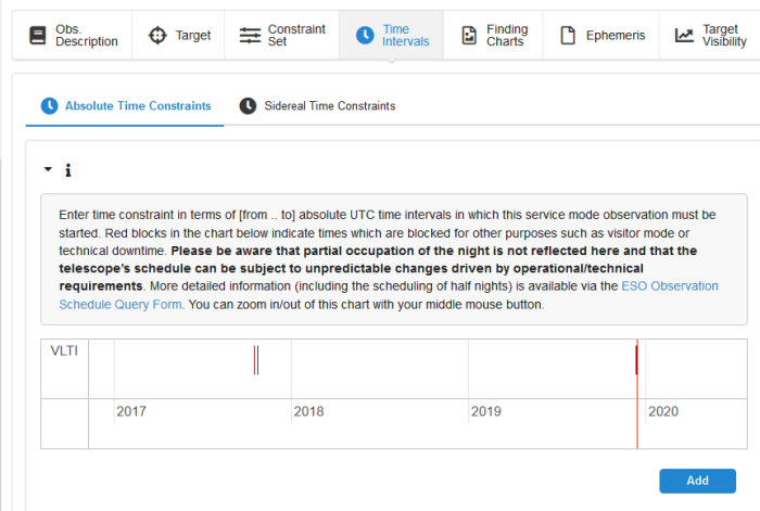
Absolute Time intervals:
Absolute time intervals should only be used if there is a scientific reason for them such as imaging of variable targets or coordinated observations with other telescopes (or observatories). If an OB with an absolute time interval cannot be executed within this constraint, they will irrevocably be removed from the queue (aquiring the status "Failed"). Please see
http://www.eso.org/sci/observing/phase2/SMPolicies/TimeCriticalOBfailure.MATISSE.html for more information.
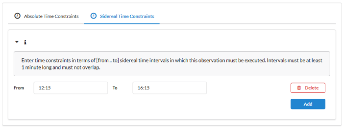
Sidereal time intervals:
VLTI OBs can have sidereal time constraints defined within which the desired projected baseline length and angle are reached and within which the observation is feasible in terms of altitude, shadowing effects, and delay line limits. It is not recommended to use LST intervals, please see the VLTI page for details. (The required information can be obtained using the visibility calculator VisCalc (maintained by ESO, but also using ASPRO, maintained by JMMC). Under the Sidereal Time tab you must specify this constraint on the the LST range. Here, because we plan to image the surface of a large star (Type of interferometric observation: imaging), we leave the LST constraints undefined. The uv-coverage will be optimized by the observing tool at Paranal).
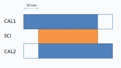
If we want to define specific LST intervals anyway, we need to make sure that each OB in the concatenation remains executable (i.e., target not setting, being shadowed by an UT, nor requiring an impossible delay line position) once the first OB in it has been sent to the telescope. This nust be done as shown below with the calibrator LSTs extending 30 min before and 30 min after the science LST interval for the two calibrators, respectively. (The white boxes indicate optional 30 min extensions to indicate executability in case of having to swap calibrators at the telescope.)
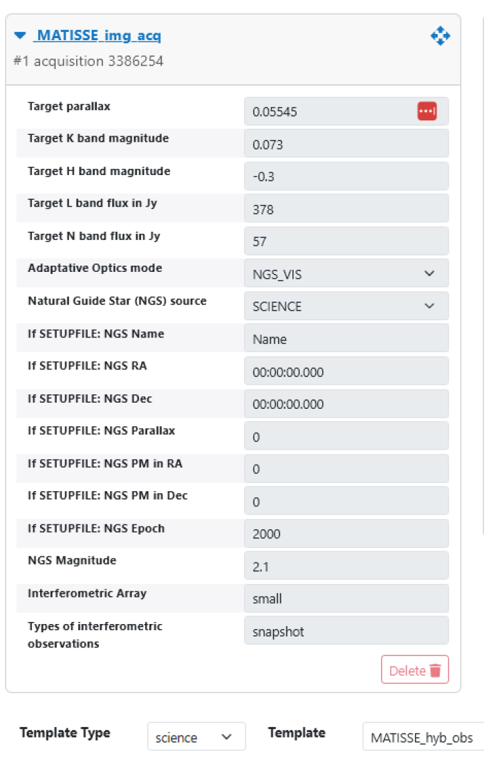
3.1.4 Defining the observing description:
We will now add the templates needed for the observation sequence, including necessary calibrations. Select the tab "Obs. description" and click the "Add" button at the bottom right of the window, making sure that the selected template is "MATISSE_img_acq". In the template, please enter the K-band magnitude of the target. The values for "RA/DEC of guide star if COU guide star is setupfile" are used in cases where the science target is not bright enough to serve for coude guiding and an off-axis guide star is provided. In that case, "COU guide star:SETUPFILE" is chosen. The parameter "GS mag" is set to the GAIA RP magnitude of the target that is used for Coude guiding, whether it is the target itself or an off-axis guide star.
Array configuration:
The configuration is defined in the acquisition template, and chosen from 4 sizes (small, medium, large and extended).
The type of interferometric observation should also be selected. Please see the page on recent changes for VLTI observations for more information.
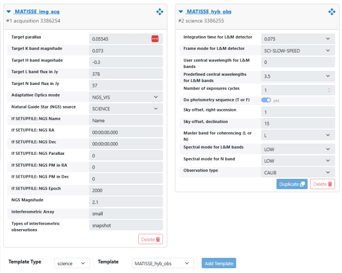
Click the "Add" button again, making sure the selected template name is "MATISSE_hyb_obs".
The example OB shown below is for the science OB! Whether an OB is SCI or CAL is selected by "Observation type" in this template.
Here, we want to observe the target in the LM and N bands. Because the target is much brighter in the L band, we choose this band for the coherencing ("Master band for coherencing"). Since we want to use the low spectral resolution mode and the target is very bright, we choose the SCI-FAST-SPEED frame mode (see the Table 4 of the Template Manual for more details). The DIT must be set to 0.020 for this combination of spectral and frame modes.
As we also simultaneously record data in the N-band, and want to make scientific use of these data, we set "Do photometry sequence" to "yes" so that the pipeline will be able to normalize the correlated fluxes and compute a visibility. For medium and high spectral resolution modes with SCI-SLOW_SPEED read-out, the full detector cannot be read and therefore you must, in these cases, specify the central wavelength for the L band.
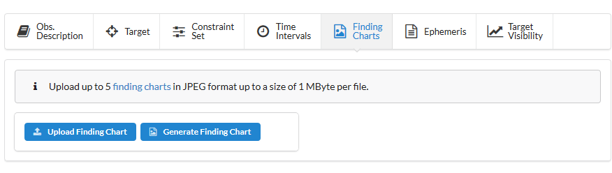
3.1.5: Attaching Finding Charts
Now that you have completed the definition of the OB, you have to attach one or more Finding Chart(s) to the OB. The Finding Charts must be prepared as jpeg-files and must fulfill all general and MATISSE specific requirements for finding charts. You can use any tool of your choice to create the Finding Charts in jpeg-format. p2 now also offers to create a finding chart by click of a button (see below).
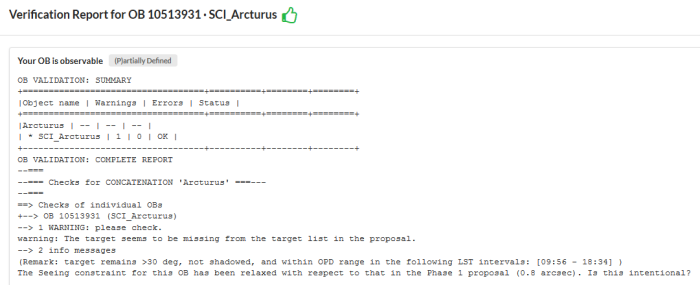
3.1.6: Checking the OB
It is recommended to check the OB definition using the "Check" button on the taskbar near the top of p2. A report will be produced, identifying any problems present, and providing information about the LST range during which the target is observable with the currently selected telescope quadruplet.
Please note: in this example, the following verification report does not pertain to the above OB defintiion for technical reasons related to the turorial account!
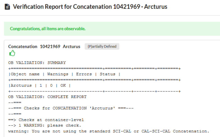
3.2: Completing the concatenation and verification
Having completed the CAL-SCI sequence, you could add another CAL OB if you want to check the consistency of the calibrator observations. You can save yourself some time after having added the science OB by selecting the calibrator OB and selecting the "Duplicate OB" option under the "Edit" menu (top task bar). This will create a copy of the selected OB and add it at the end of the current concatenation. You would still need to adapt the LST intervals though to comply with the aforementioned rules.
It is recomended at this stage to check the concatenation itself using the same "Check" button we used for the verification of a single OB, but after selecting the concatenation in the left window of p2. Even if the individual OBs check out OK, the verification of a concatention will additionally check the LST intervals in relation to each other. You may receive a wrning message for the CAL-SCI concatenation since it is non-standard; either way, CAL-SCI or SCI-CAL is OK.
4: Certification and notification
The completed concatenation is already in the ESO data base thanks to the p2 web data base interface, but it has to be certified before being ready for execution. Certification includes verification, but also sets the status of the concatenation (or OB) in the database to one which prevents modification by the user. This is to allow your support astronomer to review your OBs. Additionally, certification also checks if you have prepared the Readme information. Once you certified all concatenations of your run, you select your run and click the "Notify ESO" button. This will trigger the email to your support astronomer that your run is ready for review. For more information, see http://www.eso.org/sci/observing/phase2/p2intro/p2Features.MATISSE.html.