
UVES p2 Tutorial
This tutorial provides a step-by-step example of the preparation of a set of OBs with UVES, the UV-Visual Echelle Spectrograph at the ESO-VLT. The specifics of this tutorial pertain to the preparation of OBs for Period 101 onward. Please note that all the figures shown below can be clicked on to get higher resolution versions.
To follow this tutorial you should have familiarity with p2 : the web-based tool for the preparation of Phase 2 materials. Please refer to the main p2 webpage (and the items in the menu bar on the left of that page) for a general overview of p2 and generic instructions on the preparation of Observing Blocks (OB). Screenshots for this tutorial were made using the demo mode of p2, but should not differ in any way from one's experience in preparing your own OBs under your run.
0: Goal of the Run
In this tutorial we will prepare OBs for a simple example observing run, consisting of high resolution spectroscopy of Eta Car (RA(2000) = 10:44:39.1, Dec(2000) = -59:37:44). The sample OBs will illustrate the use of a variety of features of p2 and the kind of decisions to be taken at the time of preparing in advance an observing run, as well as some aspects that are specific to the preparation of OBs for UVES. In this imaginary observing program, we wish to observe Eta Car with two perpendicular slit orientations, and the two observations must be taken in immediate succession.
1: Getting Started
The Phase 2 process begins when you receive an email from the ESO Observing Programmes Office telling you that the allocation of time for the coming period has been finalized and that you can view the results by logging into the User Portal and clicking on "Check the time allocation information" (within the Phase 1 card). Note that the username and password that you need to use for the User Portal are the same as those you will use to prepare your OBs.
You follow the instructions given by ESO and find that time was allocated to your run with UVES. Therefore, you decide to start preparing your Phase 2 material. First, you collect all the necessary documentation:
- The UVES User Manual.
- The UVES Templates Reference Guide.
- The VLT Service Mode instructions.
- The p2 documentation referred to above.
2: Making OBs
2.0: p2
For the sake of this tutorial, we will use the p2 demo facility: https://www.eso.org/p2demo
This is a special facility that ESO has set up so that users who do not have their own p2 login data can still use p2 and prepare example OBs (for example, while writing a proposal to get the overheads right!). You cannot use it to prepare actual OBs intended to be executed. When you prepare such OBs you should use your ESO User Portal credentials for p2 (with http://www.eso.org/p2).
After directing your browser to the p2 demo facility the main p2 GUI will appear as follows:
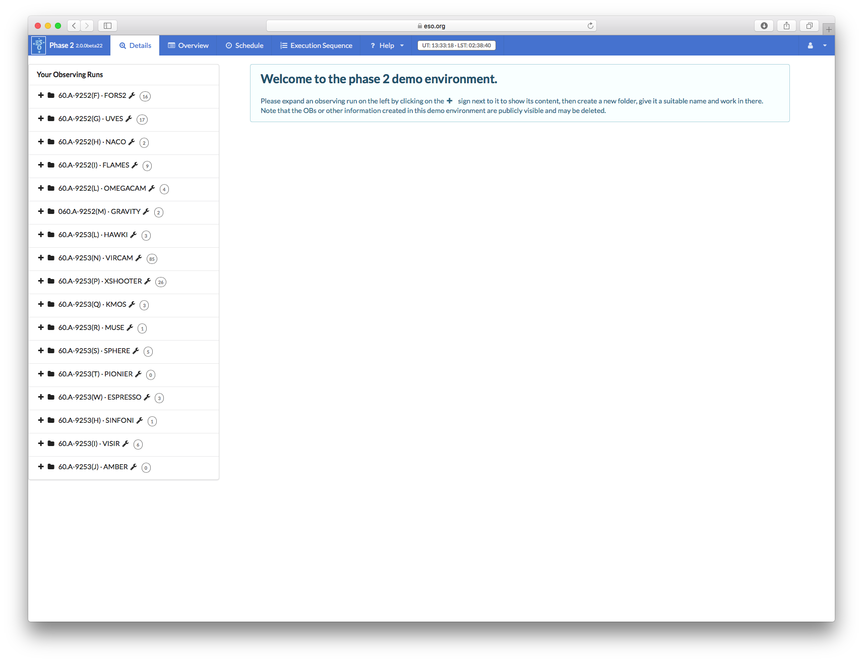
Runs for a number of instruments appear in the lefthand column, since the p2 demo facility is used for all of them. Similarly, if you log into p2 (instead of p2demo) with your own ESO User Portal credentials, you will get the list of all the runs for which you are PI, or for which you have been declared as a Phase 2 delegate by the respective PI(s).
Open the folder corresponding to the UVES tutorial run, 60.A-9252(G) by clicking on the + icon next to it. In this tutorial we assume that time was allocated in Service Mode. This is indicated by the small wrench icon that appears next to the RunID. "Inside the run" you will see (at least) one folder, called "UVES Tutorial". That folder contains the final product of the tutorial you are now reading. You can refer to the contents of that folder at any time, perhaps to compare against your own work.

You can now start defining your observations. In the p2 demo you must first start by creating a folder, within which you will put your own content. Because the p2 demo is online and accessible to anyone you may see folders belonging to other people here, though after-the-fact cleanup is possible and infact encouraged. Your screen should look like this after you pressed the folder icon:
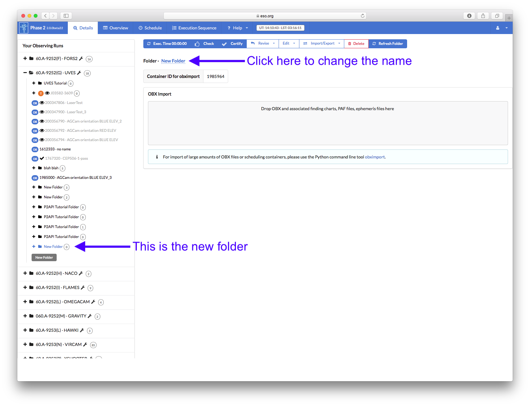
You can give the folder a new name by clicking on the blue 'New folder' text on the top, in this tutorial the name will be "The Tutorial", but you can set the name of your folder to be (almost) anything you like.
2.1: Creating OBs
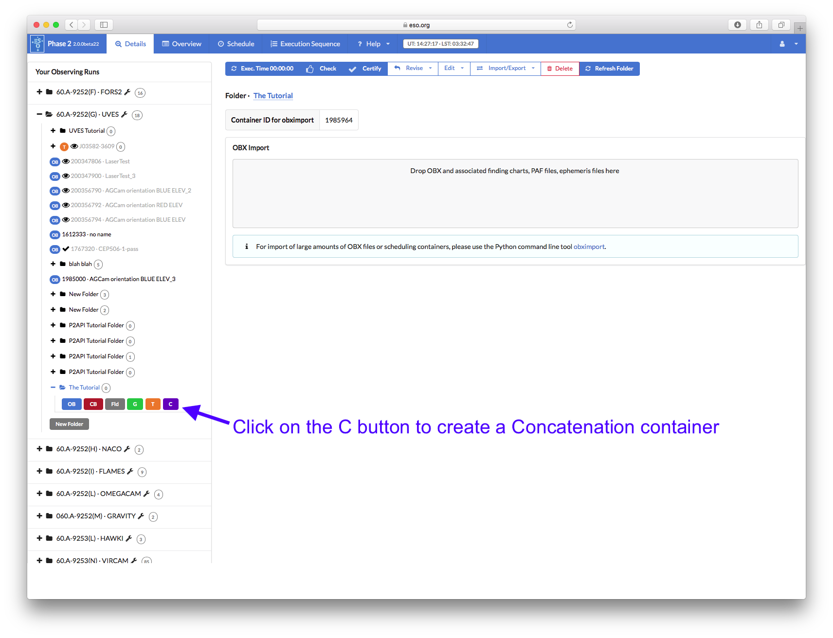
You can now start creating your OBs. Since we want our two OBs to be executed in sequence, we must define them inside a Concatenation container. Open the new folder you created by clicking on the + icon next to it and then click on the purple C icon to create a Concatenation container.
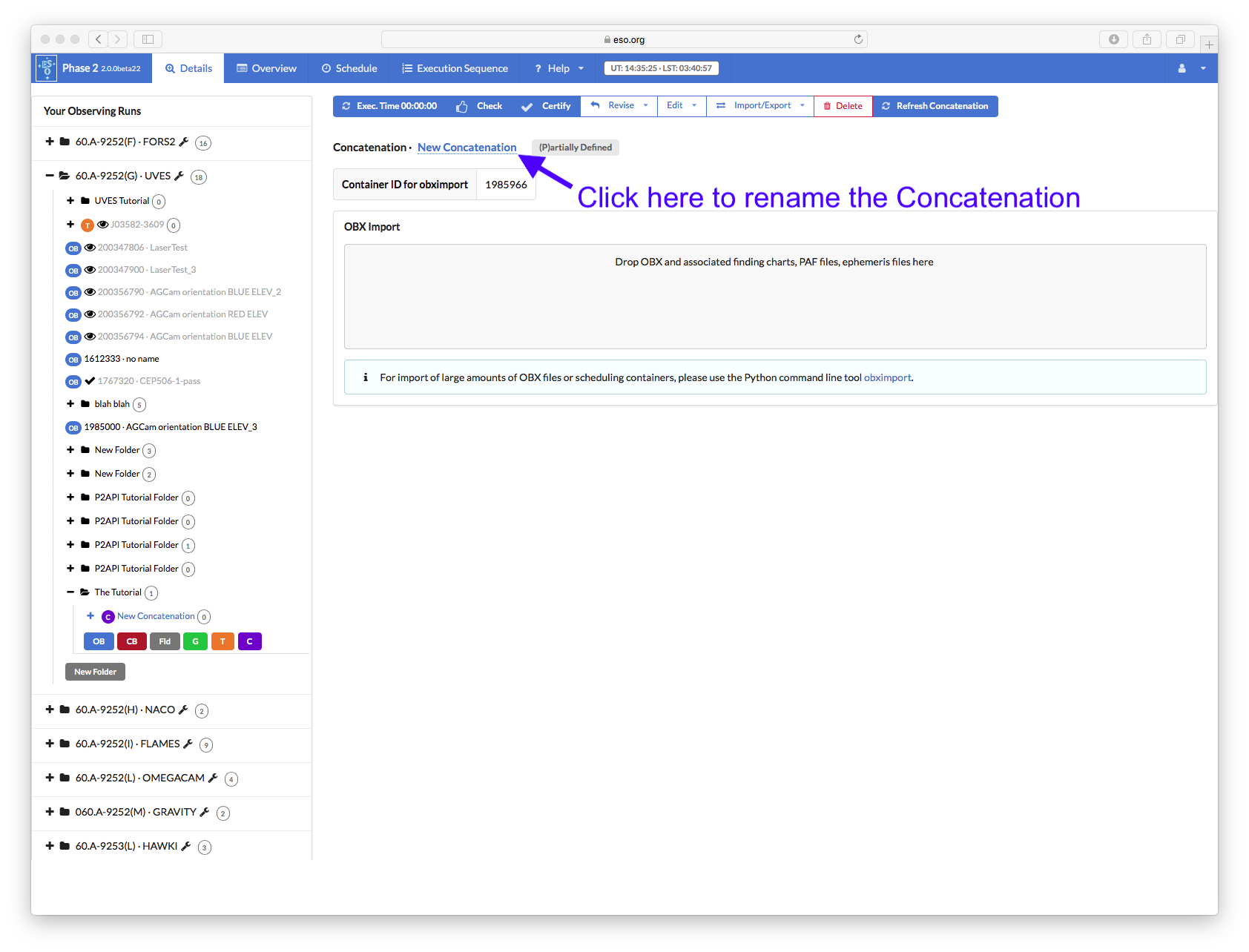
The newly created Concatenation container will automatically be selected and displayed in the main part of the window. Click on the blue name field near the top to rename the Concatenation to "eta Car at 37.5 and 127.5 deg":
To create the first OB, open the Concatenation by clicking on the + icon next to it and then click on the blue OB button of the Concatenation.
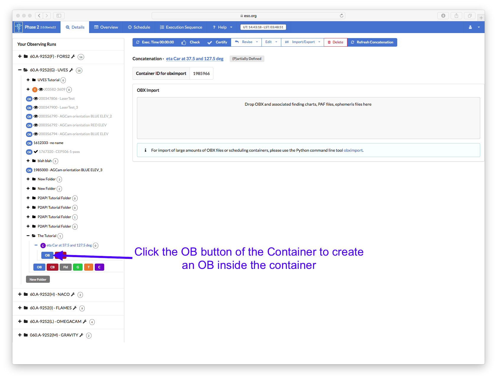
This creates the OB inside the Concatenation and it will be automatically selected and displayed in the main part of the window.
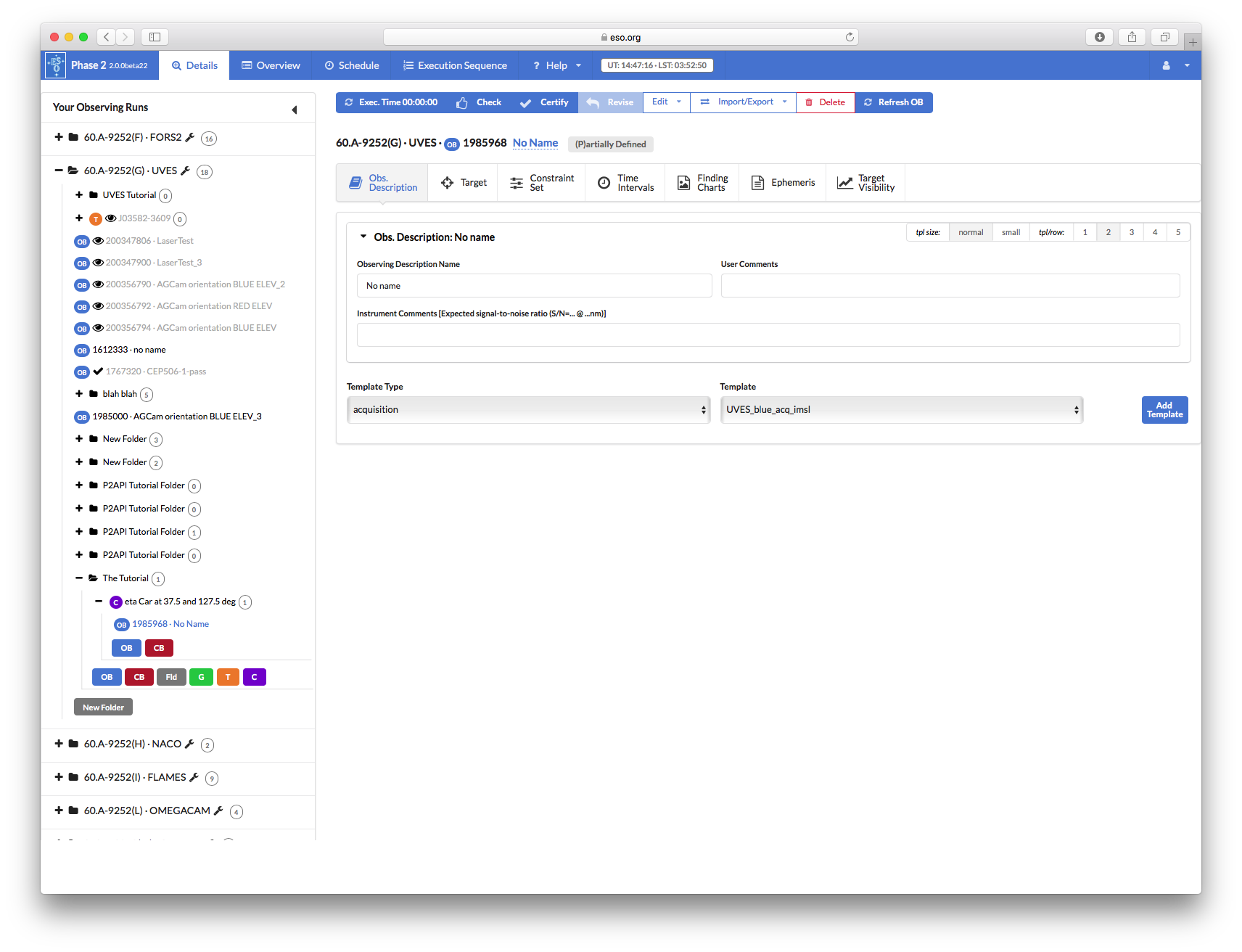
It is always a good idea to give meaningful names to OBs, so that you can browse through the list and easily recognize them. In our example, we will define OBs to take spectra of Eta Carinae using UVES Blue Arm with two different slit position angles; for this reason we will call the first OB "eta Car at 37.5 deg" by renaming it as we did for the Concatenation.
We could now also create the 2nd OB we will need, but it will be more efficient to complete the fisrt OB, duplicate it, and then just change the few things that need to be changed in order to observe at the two different position angles.
2.2: Setting the target information
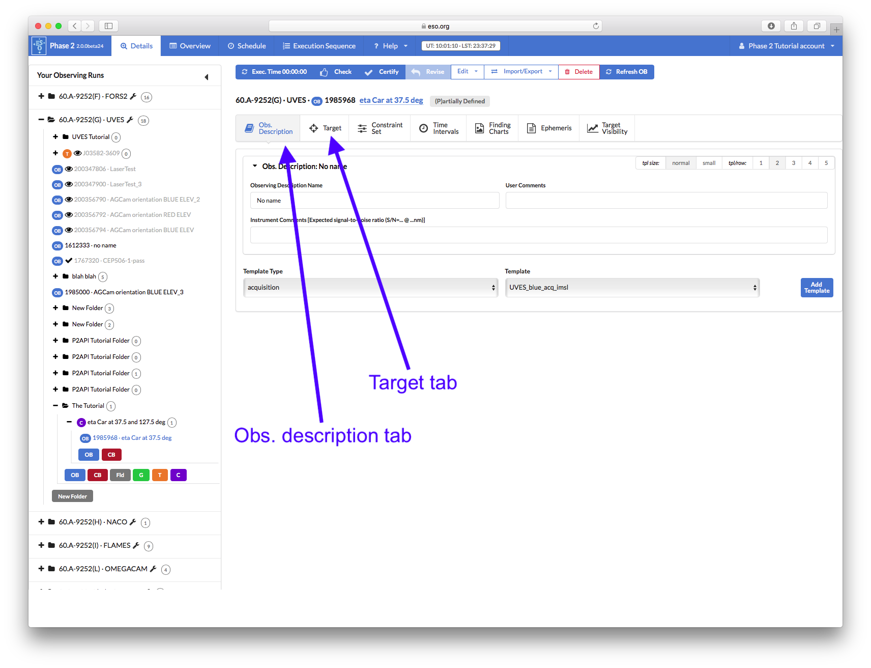
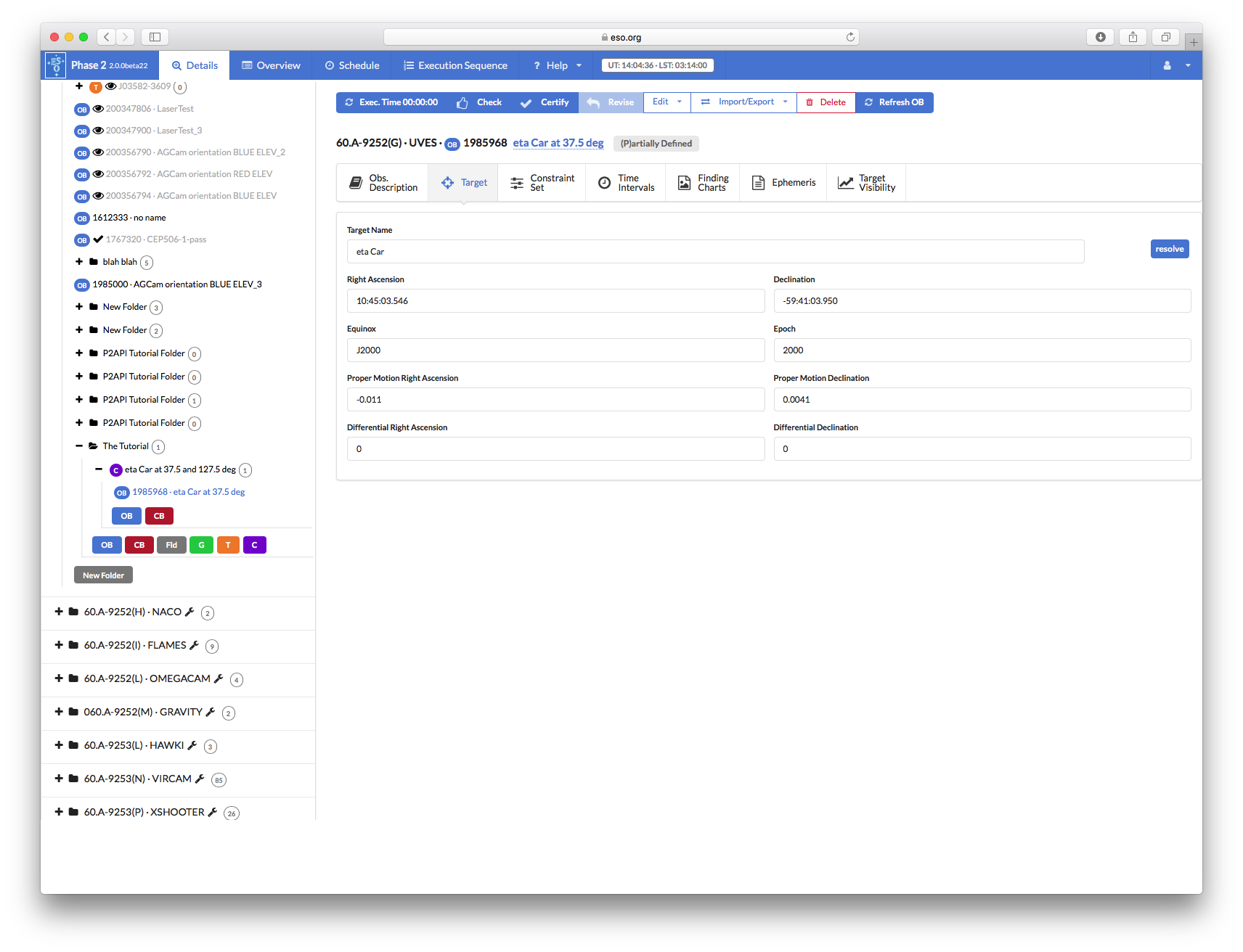
By default, the newly selected OB is displayed in the "Obs. Description" tab. To enter the target information, click the "Target" tab near the top of the window. In the Name field, type the target name "eta Car". In the Right Ascension, Declination fields, type the ICRS or FK5 coordinates. Since the coordinates are given for both Equinox J2000 and Epoch 2000, leave these fields with their default values. Wherever possible provide the Proper Motions of target, preferrably from Gaia DR2 (or newer) -- remember the units required in p2 are arcsec/yr where as most catalogues list milli-arcsec/yr. Differential tracking of the telescope is not needed for eta Car since this is not a moving Solar System target. Therefore, you can leave the last two fields in the Target tab set to their default values of zero.
2.3: Setting the constraint set
if your programme is in Visitor mode, you can ignore this section since you do not need to set the constraints for Visitor Mode OBs, but as stated in Section 1, we assume for the purposes of this tutorial that the program has been allocated time in Service Mode. You thus need to specify a constraint set for these tutorial OBs. You can do this by clicking on the Constraint Set tab and filling the fields accordingly.
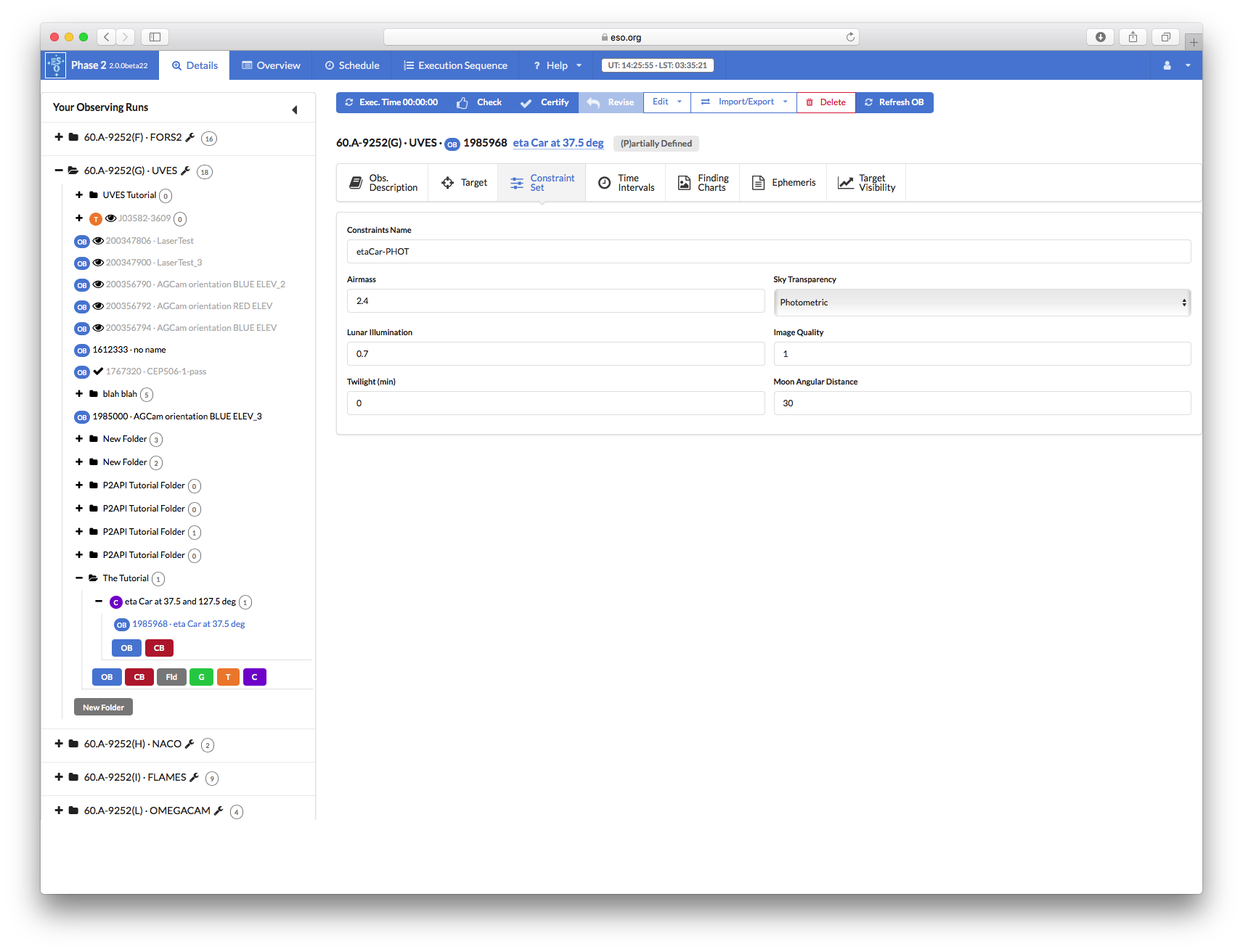
First, give a descriptive name to the constraint set about to be defined. In this case we choose "etaCar-THIN" for the Name field.
Your actual constraints then need to be set to be compatible with what you specified in your Phase 1 proposal, and at the same time consistent with the scientific goals of you project and the awarded time. You should also take into account the OPC ranking of your run.
As a rule, you can not set stricter constraints than you specified in your proposal, but you can relax the constraints compared to your proposal (see the policy here). In general you should try to relax the constraints as much as possible (in order to maximise the chances for execution) whilst balancing the constraints and exposure times in order to still achieve the S/N you need to achieve your science goals.
Also consider that while we guarantee that IF your OBs are executed, they will be executed within 10% of your constraints, they could well be executed in significantly better conditions. So if you have very relaxed constraints, you may wish to consider nonetheless several short exposures, rather than one long exposure, in order to avoid the possibility of saturation in case the OB(s) is(are) executed in significantly better conditions than the specified constraints -- Alternatively, you can note in your README strategies that the observatory could employ to avoid saturation in such cases (e.g. "If executing in significantly better conditions than the constraints please decrease expsoure times to avoid saturation whilst maintaining the targeted S/N.")
Since in your proposal you specify "Seeing", i.e. the image quality at the zenith in V-band, but in your OBs you must specify Image Quality at he wavelength of observation, the number you put in the Image Quality field of the OBs will not in general be the same as the Seeing value you specified in the proposal. In general for observations bluer than V-band you will need to specify a poorer image quality than the Phase 1 seeing you specified, while for observations redder than V-band, you can often specify and Image quality constraint better than the Phase 1 seeing you specified.
You can use the ETC to check what is the appropriate Image Quality constraint to specify for the phase 1 seeing you specified. it is also often useful to experiment with the ETC with different combinations of airmass, moon illumination and distance, sky transparency and perhaps image quality to see how to best optimise the probability for successful execution of your OBs.
Alternatively you can also use the Check function of p2, which will tell you if you have specified an Image Quality that is not consistent with your Phase 1 seeing, though you can't do this till the OB has at least a basic complete definition (see below).
So having experimented with the ETC for our present case we set the constraints as follows in order to achieve our science goals: Sky Transparency = "Variable, thin cirrus", Airmass = 2.4, Image Quality = 1.6, Lunar illumination = 1.0, Twilight (min) = 0 and Moon Angular Distance = 30 (degrees).

2.4: Setting time intervals
We will assume now that the spectroscopy of Eta Carinae has to be obtained during the period Feb 10 to Feb 15 2019, since you will have simultaneous observations at other wavelengths during that time interval. You can specify this by configuring time intervals in the Time Intervals tab.
p2 will present a representation of the allocation of nights at the telescope (unfortunately this functionality doesn't work in the p2demo environment).
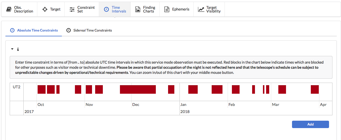
Red blocks represent nights that are not scheduled as full nights of Service Mode, so you should aim to have as many as possible absolute time intervals outside the red blocks. It is possible that serivce mode OBs can be executed during red blocks (e.g. because the particular night is a half-night of Service Mode) but you should not rely on this possibility just based on this view. More detailed information (including the scheduling of half nights) is available via the ESO Observation Schedule Query Form (see below). Please bear in mind though that the schedule does evolve during the period according to operational needs. Therefore include all possible absolute time intervals during the period, even if they fall entirely within red blocks.
To add an absolute time interval, just click the blue Add button below and to the right of the schedule. This will add a new "from" and "to" pair of fields, you can adjust the from and to dates and times by typing directly in the fields or by using the calendar (and following time) widgets to the right of each field.
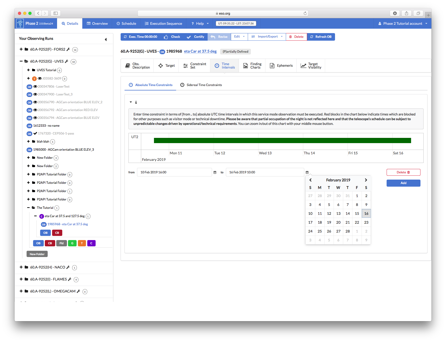
Once a valid interval has been entered it is displayed in the schedule view as a green block.
It is important to keep in mind that Absoute Time Intervals represent the intervals during which the OB can be started, not the intervals during which the OB must be started and finished. For an interval like the one above this is not really an important distinction. But in certain situations it can be, for example imagine you wish to obtain spectra before, during and after a planetary transit. If you have (say) 4 hrs of OB(s) (with an approved waiver of course), and the transit lasts 3hrs, and you need at least 15mins of observations before and after the transit, then you will have just a 30min long window, starting 45+6mins before and ending 15+6mins (remember there is ~6mins of overhead from the start of an OB before any science spectra are taken) the transit during which the OB must be started, and the Absolute Time Interval(s) must be set to these 30min intervals.
Each OB can have multiple time intervals (in general the more the better to improve the chances of execution). Just click the Add button to add additional interval(s). Each interval also has a delete button which allows you to remove intervals one by one.
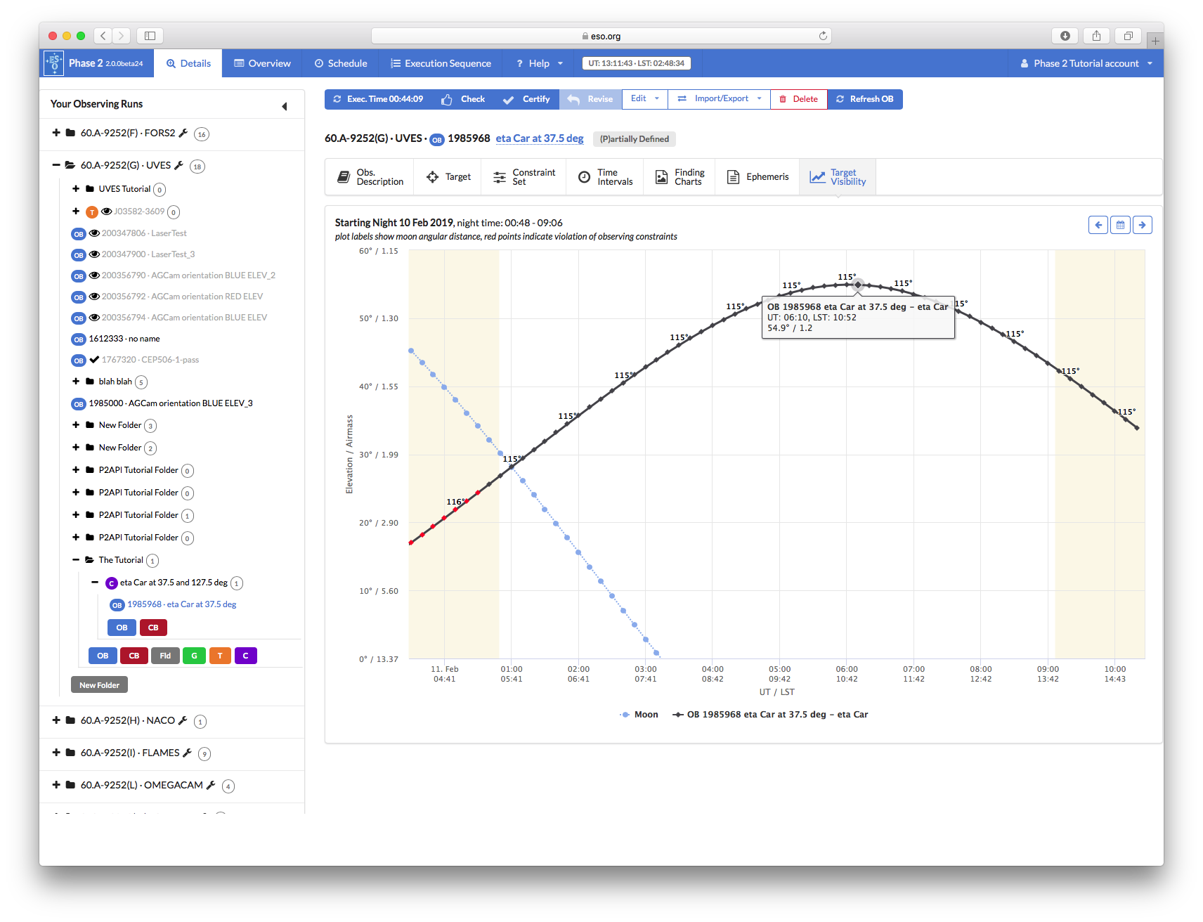
The Target Visibility tool accessible via the Target Visibility tab is useful to check that your target is actually observable within your defined constraints during your defined time intervals.
Note that all time critical aspects (absolute time intervals and timelink containers) must also be explained in the section on "Time Critical Aspects" of the README (see the README tutorial here). Note, no need to list the specified Absolute Time Intervals, just explain why they are needed (e.g. for the planetary transit example above, 30min long Absolute Time Intervals specified in order to start the observations at least 15mins before the start of the 3hr long planetary transit and to finish at least 15mins after the end of the transit).
For more information on entering time constraints and how to use TimeLink containers to enter relative time constraints, see the generic p2 tutoirals here.
2.5: Defining the Observation
Finally we get on to defining the actual observations.
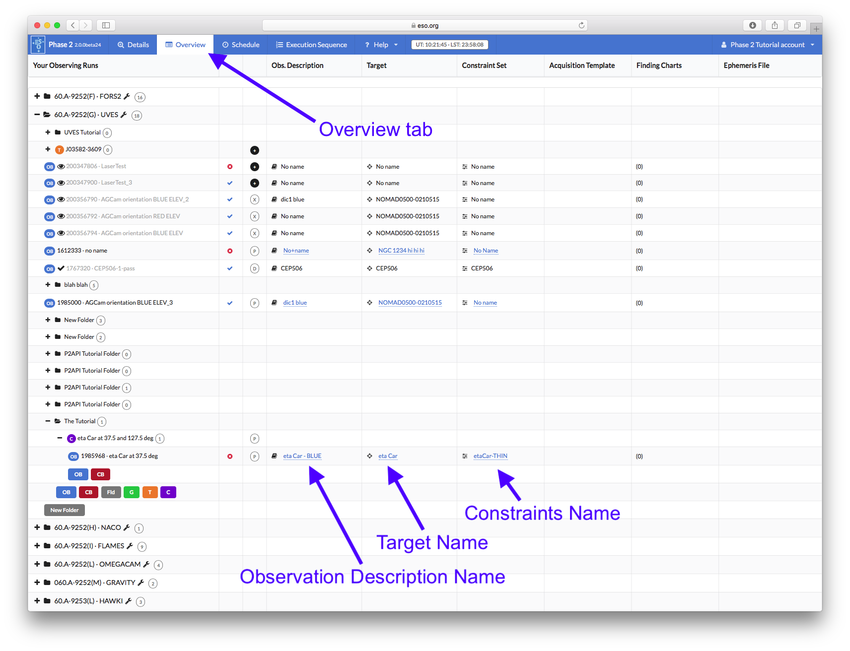
An OB is defined by a set of one or more templates that form the Observation Description, or OD for short. It may be useful in many cases to have an easy way of identifying an OD, like when having observations of a number of targets performed with identical instrument configurations and exposure times. The Observing Description Name field in the Obs. Description tab allows you to define name of the OD. The OD name appears in turn in one of the columns of the Overview tab, thus allowing the identification at a glance of all OBs having ODs with the same name.
In this example OB, the OD will consist of a sequence of three spectra with increasing exposure times. We can thus appropriately name it eta Car - BLUE. We enter this name in the Observing Description Name field, and we can now see this in the Overview tab.
Now back to defining the observations, click directly on the Details tab button next to the Overview tab button.
The first template that must be part of any science OB is the acquisition template, so let us define it first. In the Template Type pull-down menu, make sure that the acquisition entry is highlighted. Now we can select the appropriate acquisition template from the Template pull-down menu on the right.
After reading the description of the templates in the UVES User Manual, you have determined that the UVES_blue_acq_slit is the acquisition template you have to use for this particular observation. You thus click on this template in the Template pull-down menu list, and then on the blue Add Template button next to it.

We now need to decide on the acquisition parameters. Since we want to acquire directly on Eta Carinae, we will leave both RA blind offset and DEC blind offset set to 0. You do not have any special requirements on the guide star, which will be selected by the telescope operator from the VLT guide star catalogue at the time of executing the OB, so we leave Get Guide Star from set to "CATALOGUE", and hence there is also no need to specify any coordinates for the guide star (so we leave Guide star RA and Guide star DEC set to 00:00:00.000).
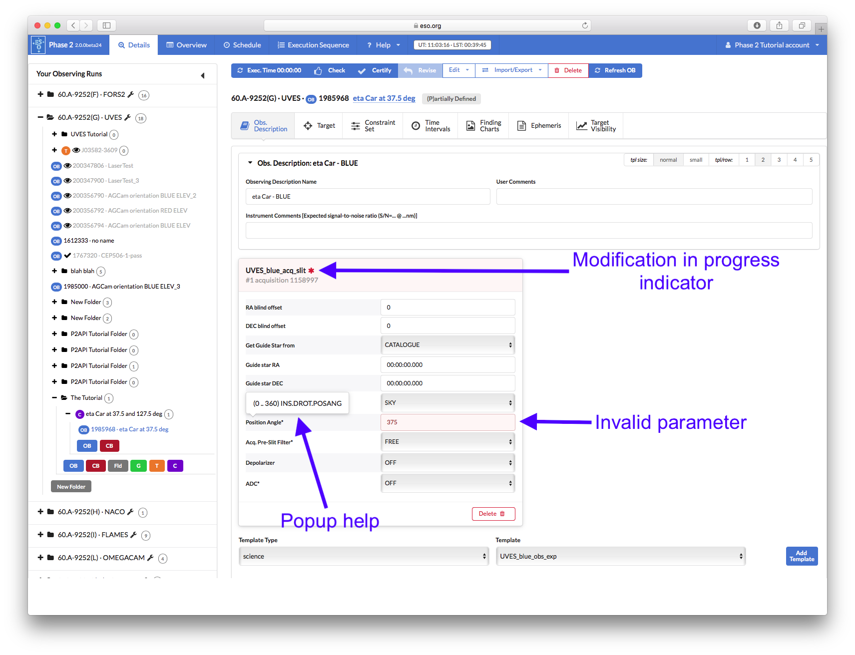
Since we want to place the slit on a position angle of 37.5 degrees, we have to set Derotation Mode to SKY and the Position Angle to 37.5.
Unfortunately we enter 375, rather than 37.5, but this is an invalid entry. This is indicated by the field turning red. Hovering the mouse over the parameter name gives a popup with the valid range of the parameter and the technical name of the parameter (as it will be specified in the FITS header of the resulting data). We also see that there is a "Modifications in progress" indicator. This red asteriks actually appears anytime you change any information in the OB. It indicates that the current state of the OB has not yet been synchronised to the ESO database. Note then that the OB is NOT synchronised as long as any entry is invalid. Note that if we would perform some other action such as "Check" while there is an invlaid parameter, the OB will first revert back to the version currently in the ESO database.
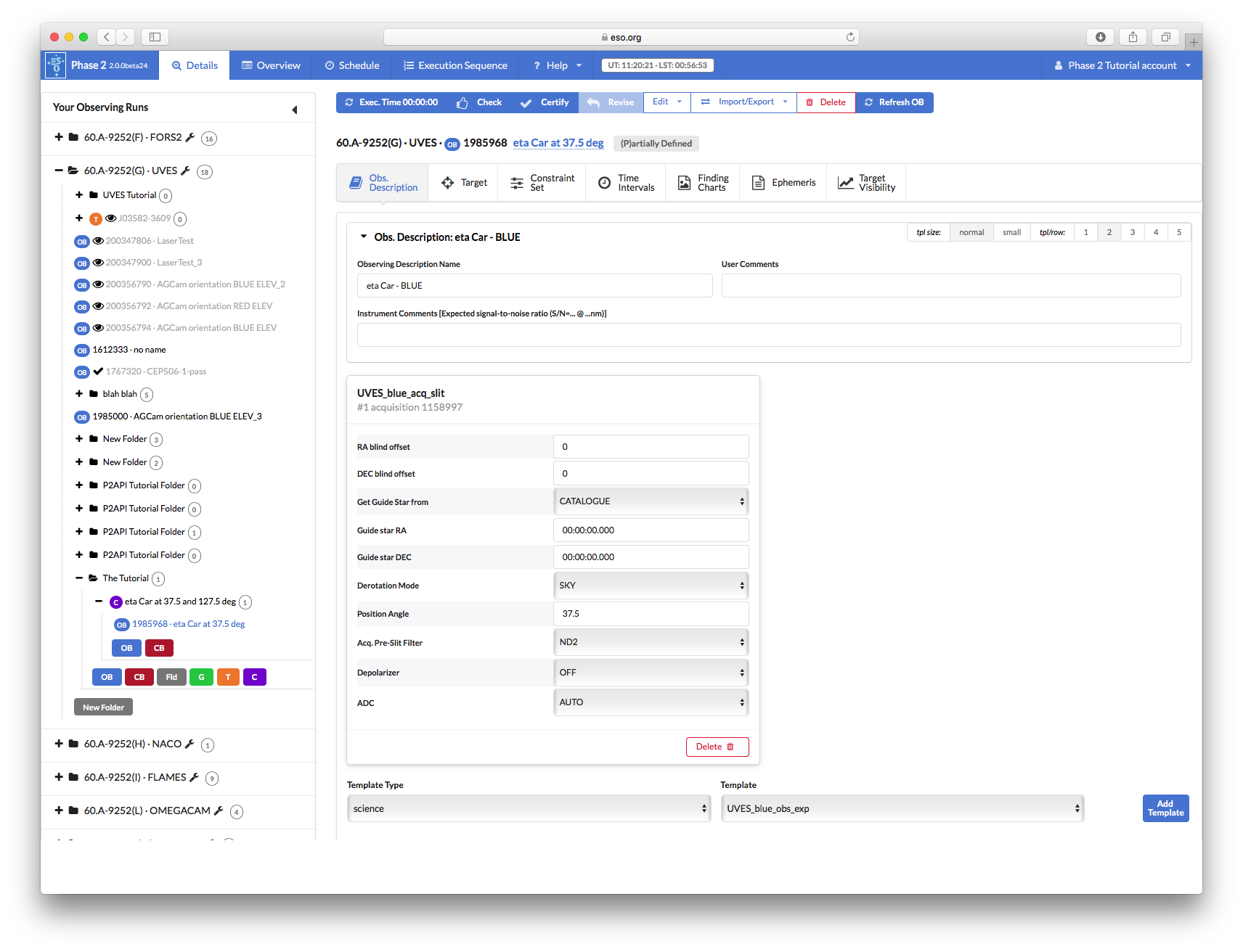
We correct the value of the Position Angle. Note that the "Modification in progress" indicator persits for about 1sec, then changes to a spinning activity indicator showing that the change is now being synchronised with the ESO database. Once synchronisation has successfully completed it should disappear.
Now we can continue with the remaining parameters. Eta Carinae is a bright star, and thus it is a good idea to use the neutral density filter ND2 as pre-slit filter for the acquisition (Acq. Pre-Slit Filter). There is no need for a depolarizer, so Depolarizer is left OFF, but we do want to limit the slit losses and therefore we want to use the Atmospheric Dispersion Corrector so we set ADC to AUTO.
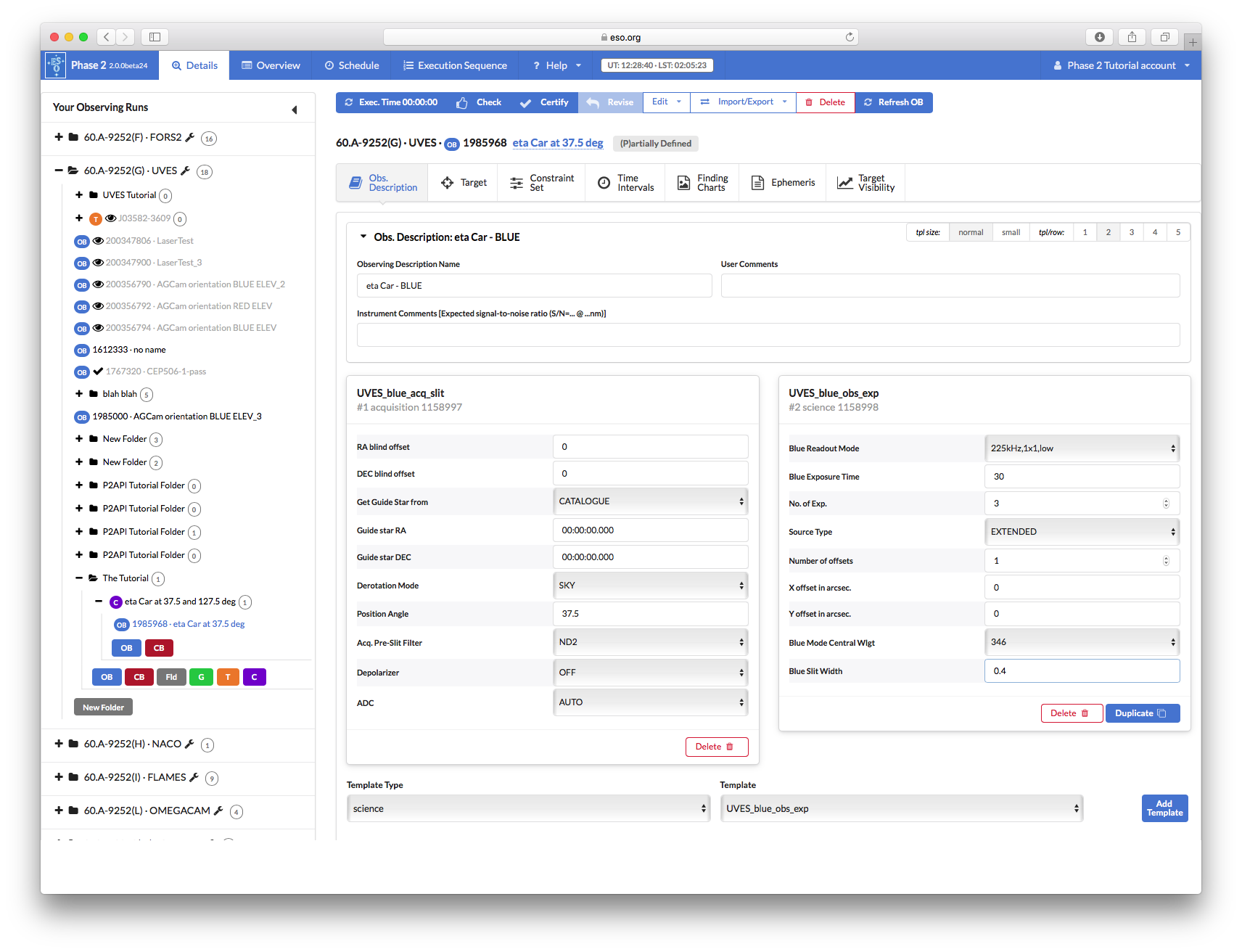
Once the acquisition is completed, the science observations begin, so the observing templates need to be attached. After checking with the manual and considering the scientific requirements of your program, you have found that the appropriate template to be used is UVES_blue_obs_exp.
From the Template Type pulldown menu, select science. Then select the UVES_blue_obs_exp template from the Template pull-down menu list, and then click on the Add Template button.
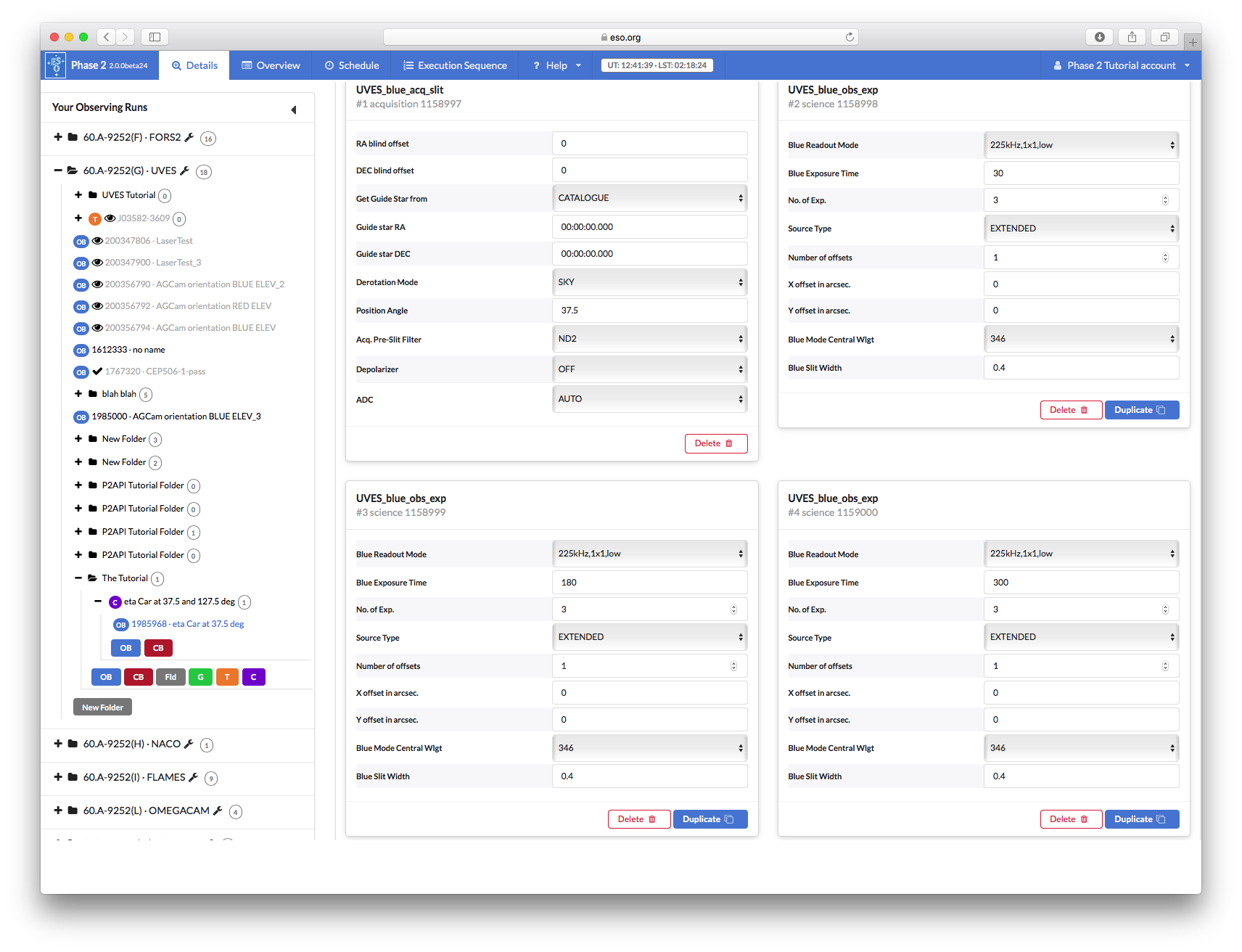
Following the recommendations of the manual, you choose to use the standard read-out mode 225kHz,1x1,low. For your scientific purposes you need to obtain 3 spectra of 30 seconds each of Eta Carinae, which is definitely an extended object. Due to the high signal-to-noise ratio you expect to achieve, you do not need to perform any offset along the slit. The default central wavelength (346) is the correct one but you want to improve the resolution as much as possible by using a narrow slit available. The set of parameters that you choose in your science template is thus as depicted below:
Since you now want to perform another two sets of observations with two different (longer) exposure times, you could select again the same template, Add it, and fill the parameters in the same way as done for the first template. However, since the parameters of these other two templates will be very similar to those of the one just defined, you can speed up the preparation by duplicating the template you just created by clicking the blue Duplicate button inside the science template frame twice. In this way, you will have produced two identical copies of the first science template in which you should now only edit the parameters that change from template to template, i.e., the exposure times, which are going to be 180 and 300 seconds respectively.
You can now compute the execution time of this OB. First scroll to the top of the page if necessary then click the blue Exec. Time button in the blue button bar near the top of the window.

NOTE: the execution time field is not updated automatically, you thus need to click on the Recalculate button to display the correct value after any modification.
Finally, to complete the OB preparation, enter the expected signal-to-noise ratio in the Instrument Comments field, using the following syntax: S/N=XYZ @ xyz nm:

2.6: Attaching Finding Charts
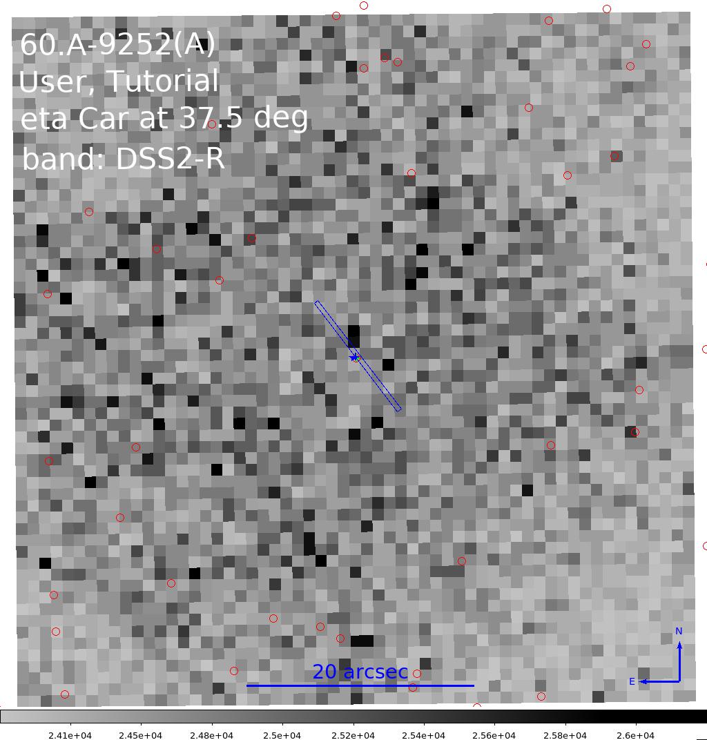
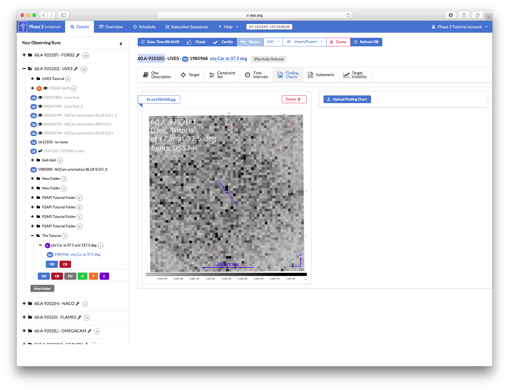
Finding charts, see the guidelines here, must be attached directly to the OBs. Select the Finding Charts tab, click the blue Upload Finding Charts button and select the pre-prepared jpeg file(s) in the file chooser (you can download the finding chart file used in this tutorial from here). Once successfully uploaded to the ESO database, they will be displayed in the p2 window.
This completes your first OB!
2.7: Making more OBs
We want to add another OB to our Concatenation in order to take a spectrum with the slit direction perpendicular to that of the first OB. Insure that the OB that you want to duplicate is selected and then click on the Edit button in the OB tool bar near the top of the p2 window, and then click on Duplicated OB in the menu that appears.
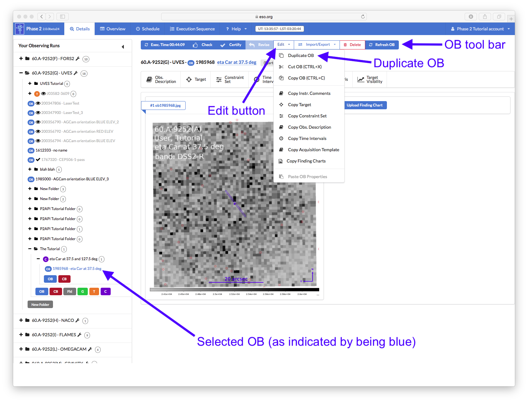
This will add an identical OB to the concatenation with _2 appended to the OB name and this new OB will be selected as the displayed OB. Rename this new OB to "eta Car 127.5deg". Click in the Edit icon, we now only need to change two things: (1) the value of the Position Angle in the acquisition as shown in the image below...
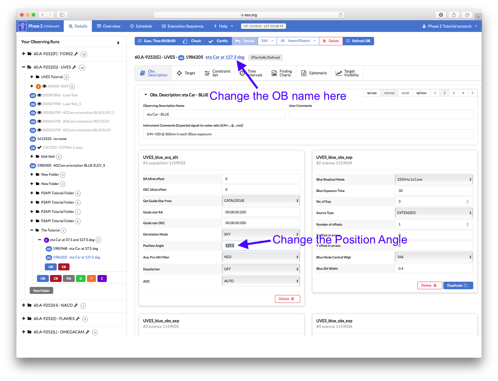
and (2) delete the exisiting finding chart...
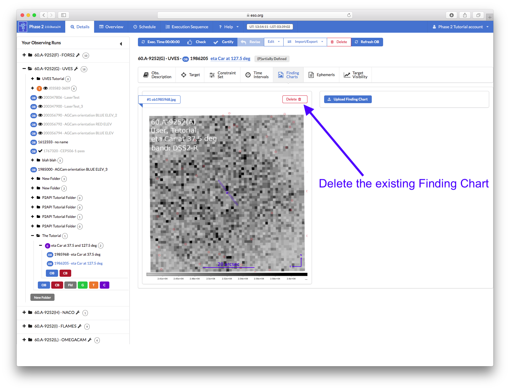
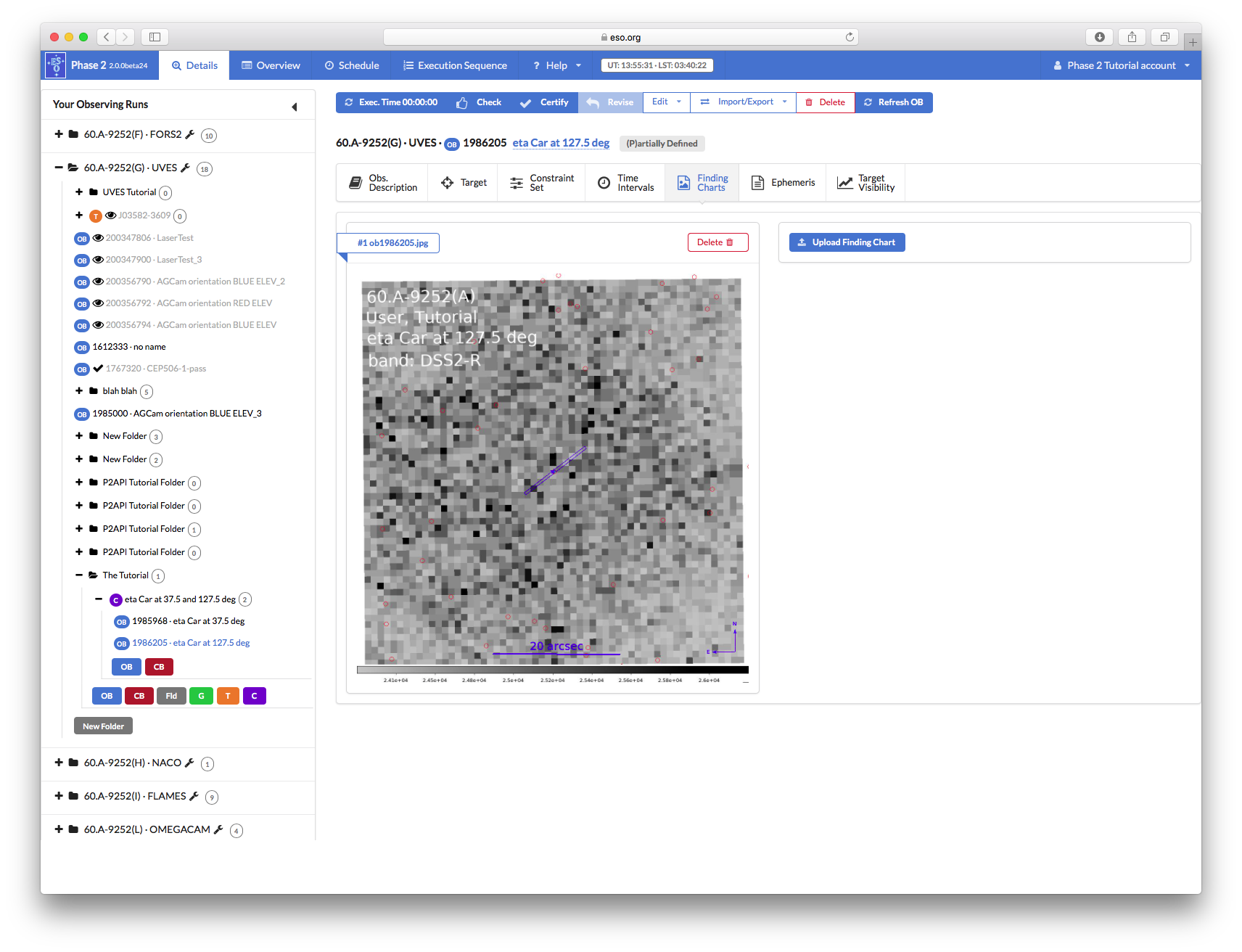
...and attach a new finding chart showing the proper slit orientation (you can download the finding chart file used in this tutorial from here).
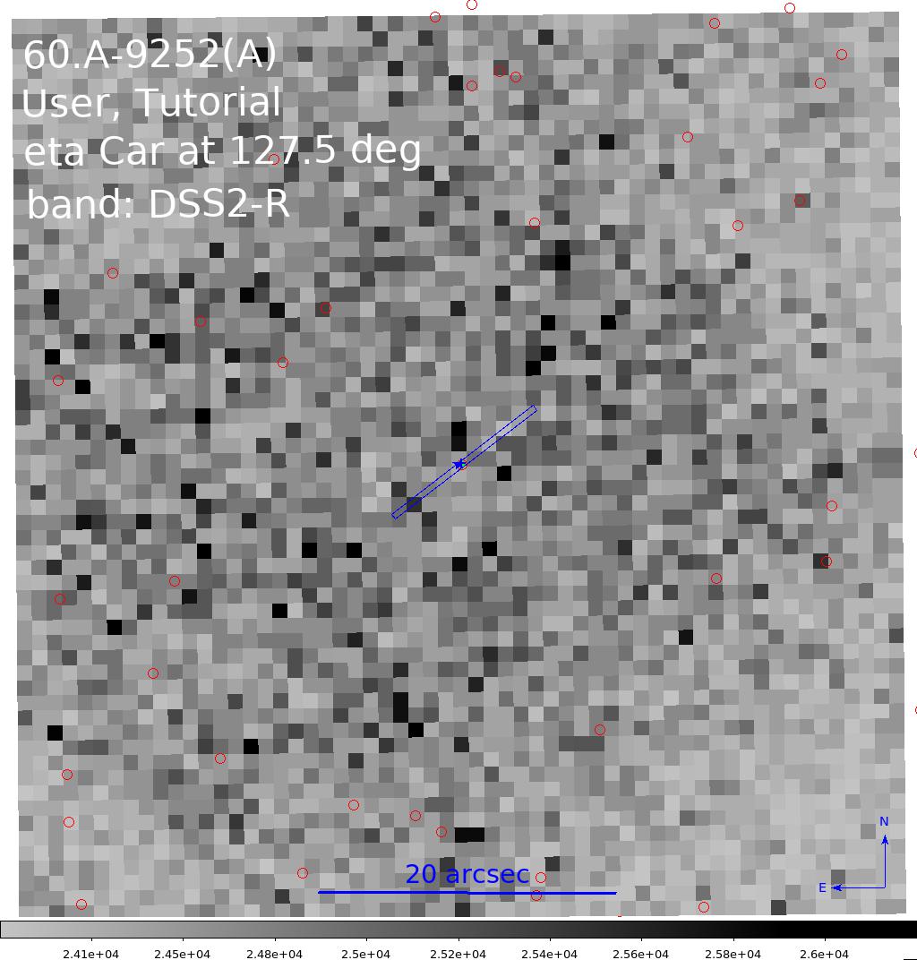
3: Finishing the preparation and submitting the OBs
Once you think that the OBs are complete and ready for execution, you should compute the execution time (to make sure it is within your allocated time) and Check the content of the OBs using the Verification Module.
If a single OB is selected, the Exec.Time button in the OB tool bar will compute the execution time of just that one OB and as if it is executed as a standalone OB, even if it is in a container, e.g. the two OBs created in the tutorial above each have execution times of 00:44:09 (as standalone OBs). If multiple OBs are selected (via shift-click or Alt-click on PC/Cmd-click on Mac), the Exec.Time button in the OB tool bar will compute the total execution time of all selected OBs as if they are executed as standalone OBs, even they are in a container, e.g. if the two OBs created above are both selected p2 will report a total execution time of 01:28:18, as if the two OBs are executed as wo standalone OBs. But if a concarenation is selected it will compute the execution as if the OBs are executed back to back, in particular you will save overheads on the acquisition if the OBs are close together on the sky, e.g. if the concatenation created above is selected p2 will report a total execution time for the concatenation of 01:22:58. And if you now select the second OB in the concatenation, you will see that it's execution time is only 00:38:49 while the first OB still has an execution time of 00:44:09.
If you are happy with the total execution time of all OBs and containers that you wish to submit, then you should Check the OBs/concatenations. As with computing the execution time, you can check individual OBs, multiple OBs, containers, multiple containers, folders and even multiple folders. For containers, running a check will perform container level checks (e.g. checking the total execution time of the container) as well as rnning checks on all the individual OBs within the container. For folders, running a check will perform checks on all OBs and containers and folders within that folder.
The Check makes detailed verifications of the structure and contents of the OBs and containers. The OBs and containers must successfully pass these checks in order to be executable at the observatory. Some errors can be accepted with an approved waiver, others simply have to be fixed in the OB(s).
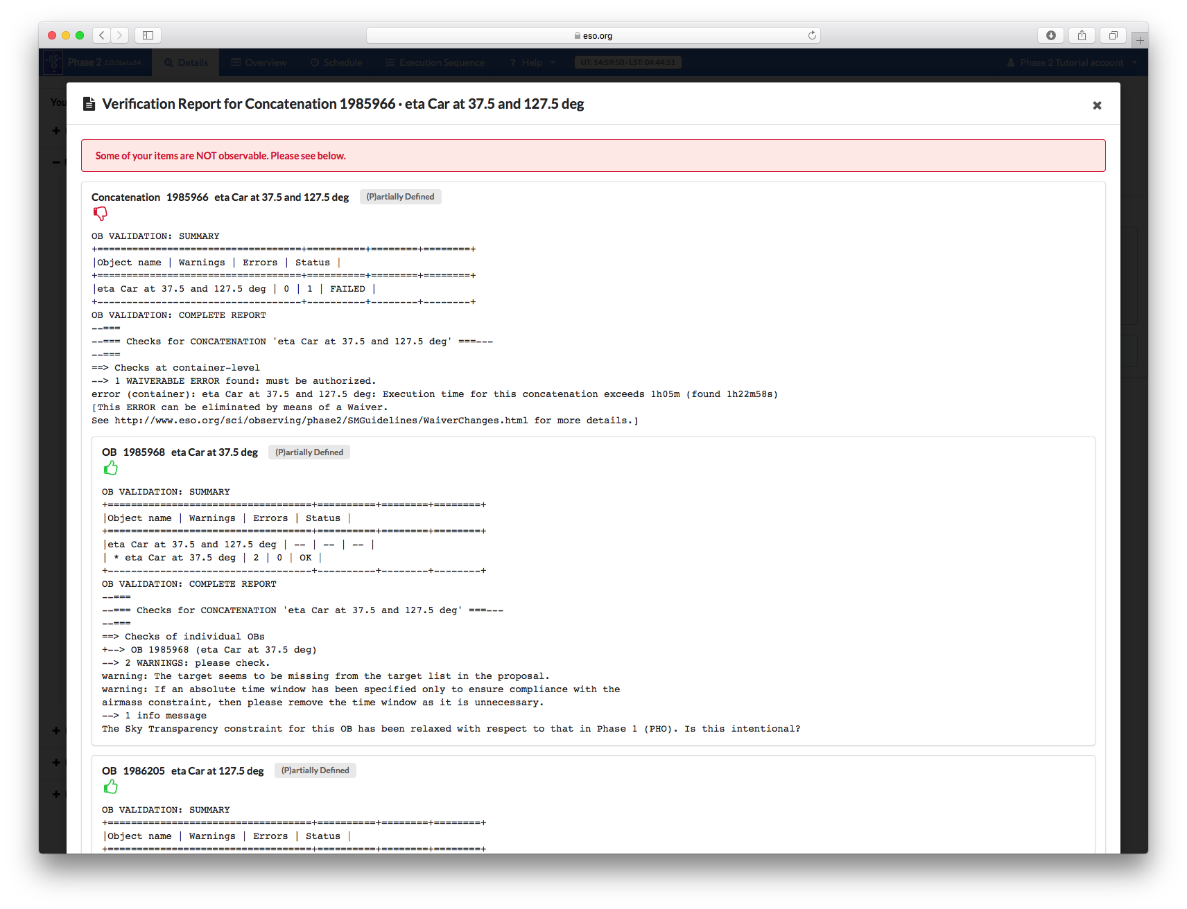
Above is the result of running Check on the eta Car concatenation created above. The individual OBs pass successfully, but the concatenation itself fails due to the total execution time exceeding 1hr. To fix this one would have to either, reduce the total execution time buy decreasing expsoure times and/or numbers of expsoures, move the OBs out of a container, but thus accept that they would probably not be executed back-to-back, or else obtain an approved waiver for a concatenation execution time of 1h22m.
This tutorial is now completed.
As already mentioned, it has certainly not covered all the observing strategies you may have foreseen for your program, but it has shown how to prepare OBs for a representative case.
To complete a Phase 2 submission you would still need to:
- Complete the README
- Certify the OBs and containers
- Notify ESO
Please see the general tutorials here which cover these topics.