
KMOS p2 Tutorial
This tutorial provides a step-by-step example of the preparation of a set of Observation Blocks (OBs) with KMOS, the K-band Multi Object Spectrograph on UT1 (Antu) of the VLT. The specifics of this tutorial pertain to the preparation of OBs for Period 105 onwards. Please note that all the figures shown below can be clicked on to get higher resolution versions. The figures show p2 as released for P105. In subsequent periods some new features, for example the waiver/change request button, were added.
To follow this tutorial you should have familiarity with p2: the web-based tool for the preparation of Phase 2 materials. Please refer to the main p2 webpage (and the items in the menu bar on the left of that page) for a general overview of p2 and generic instructions on the preparation of Observing Blocks (OB). Screenshots for this tutorial were made using the demo mode of p2 for Period 105.
0: Goal of the Run
In this tutorial we will prepare OBs for one simple example observing run.
The science case consists of spectroscopy in the HK band of lensed galaxies behind the massive galaxy cluster A1689.
1: Getting started
The Phase 2 process begins when you receive an email from ESO telling you that the allocation of time for the coming period has finalized and that you can view the results by logging into the User Portal and clicking on "Check the time allocation information" (within the Phase 1 card). Note that the username and password that you need to use for the User Portal are the same as those you will use to prepare your OBs.
You follow the instructions given by ESO and find that time was allocated to your run with KMOS. Therefore, you decide to start preparing your Phase 2 material.
First, you collect all the necessary documentation:
- The KMOS User Manual
- The VLT Service Mode Guidelines
- The p2 documentation referred to above.
One very important prerequisit for the preparation of KMOS OBs is one or more KARMA set up files, which have to be attached to the OBs. In those files the positions of the arms as well as the coordinates of the guide and reference stars are defined. KARMA also should be used to create the necessary finding charts that have to be attached to the KMOS science OBs. You can find the documentation and download page of KARMA here:
- The KARMA User Manual
- The KARMA web page
2: Science case: lensed galaxies behind A1689
Let's start with this science case. So, off you go to define those observations.
2.1: p2
For the sake of this tutorial, we will use the p2 demo facility: https://www.eso.org/p2demo
This is a special facility that ESO has set up so that users who do not have their own p2 login data can still use p2 and prepare example OBs (for example, while writing a proposal to get the overheads right!). You cannot use it to prepare actual OBs intended to be executed. When you prepare such OBs you should use your ESO User Portal credentials for p2 (with http://www.eso.org/p2).
After directing your browser to the p2 demo facility the main p2 GUI will appear as follows (or similar, since more runs are added from time to time):
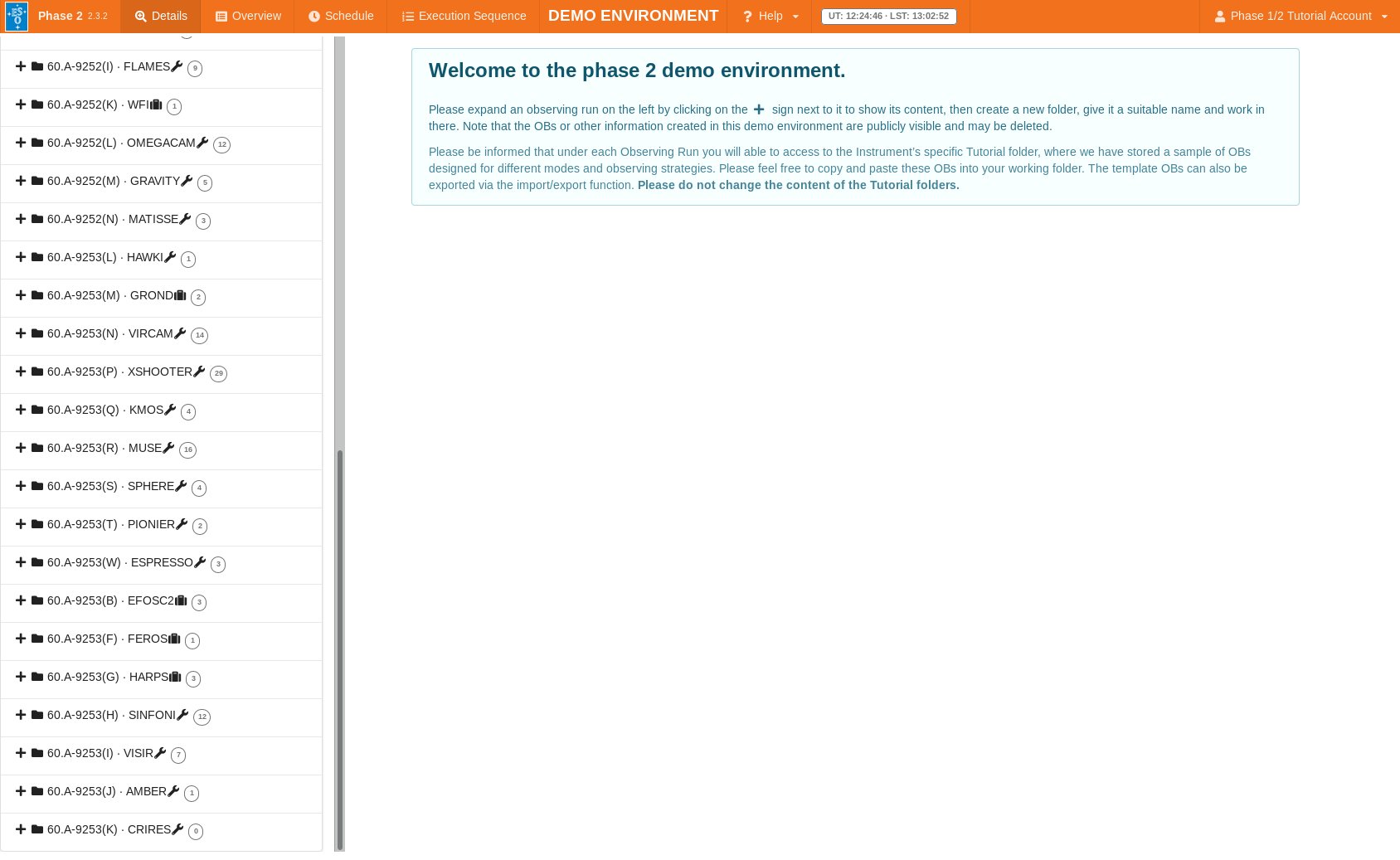
Runs for a number of instruments appear in the lefthand column, since the p2 demo facility is used for all of them. Similarly, if you log into p2 (instead of p2demo) with your own ESO User Portal credentials, you will get the list of all the runs for which you are PI, or for which you have been declared as a Phase 2 delegate by one of your colleagues.
Select the folder corresponding to the KMOS tutorial run, 60.A-9253(Q) by clicking on the + icon next to it. In this tutorial we assume that time was allocated in Service Mode. This is indicated by the small wrench icon that appears next to the RunID. "Inside the run" you will see (at least) one folder, called "KMOS Tutorial". That folder contains the final product of the tutorial you are now reading. You can refer to the contents of that folder at any time, perhaps to compare against your own work. But, please do not create your test OBs under this folder!
You can now start defining your observations. In the p2 demo you must first start by creating a folder, within which you will put your own content. Because the p2 demo is online and accessible to anyone you may see folders belonging to other people here, though after-the-fact cleanup is encouraged and possible. Your screen should look like this after you pressed the folder icon:
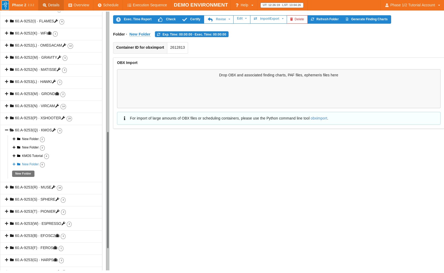
You can give the folder a new name (in this example 'My test folder') by clicking on the blue 'New folder' text on the top, and then start creating your OBs. In this science case we want to have three OBs on the same target configuration because our galaxies are faint and the S/N reached with one 1-hour OB would not be sufficient.
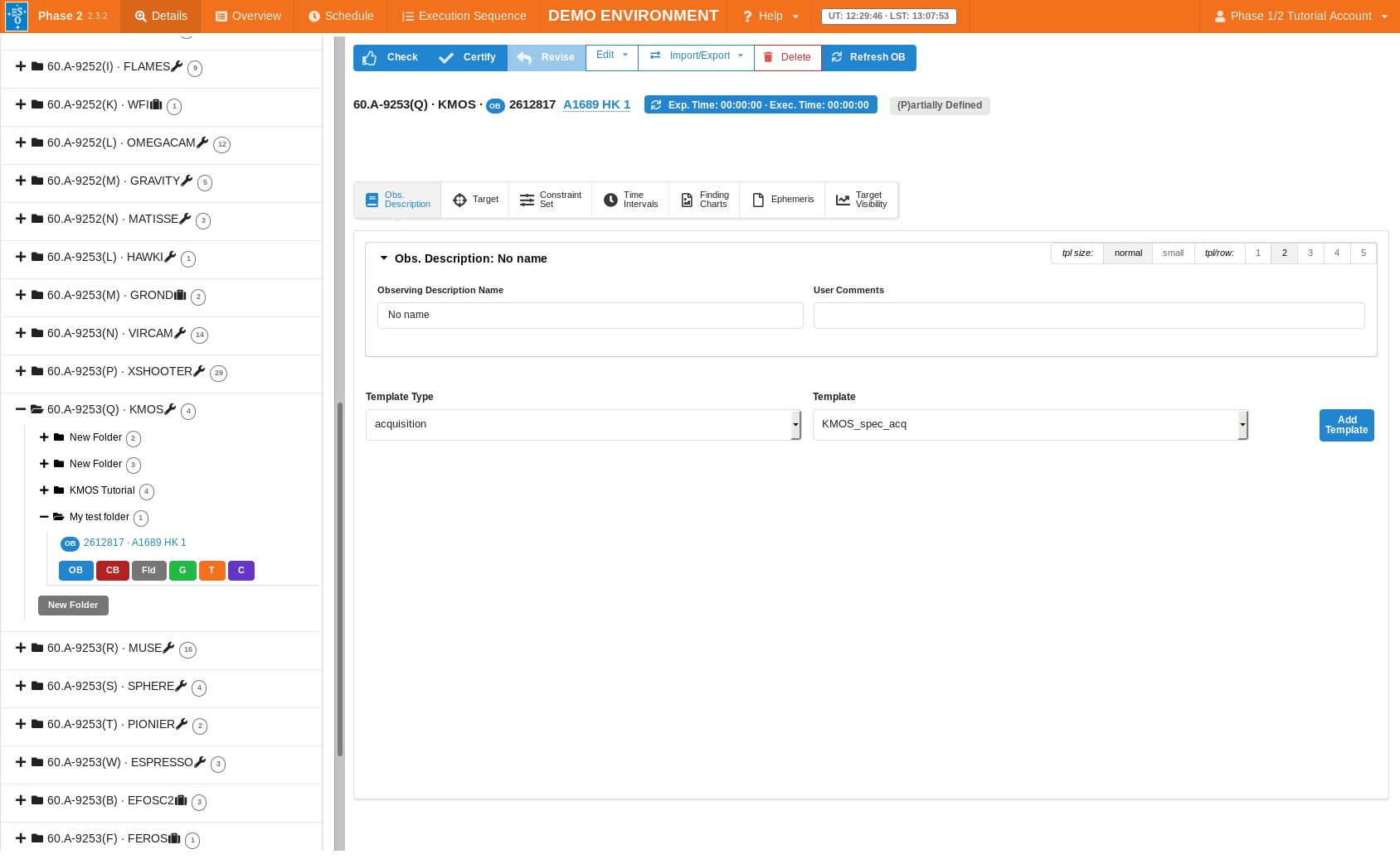
To create an OB, first select your folder icon in the left menu, then press the blue 'OB'-icon below your folder. You will now be able to edit its contents on the right hand side of the GUI. You can give the OB a name by clicking on the blue 'No name' text on the top. Let's call the OB 'A1689 HK 1'. Your screen should then look like this:
2.2: Defining an OB
2.2.1: Filling in the Basic Information
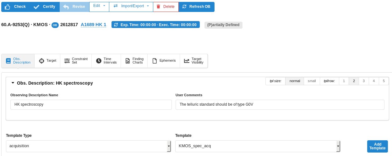
This is an OB for spectroscopy in the HK band. It may be useful in many cases to have an easy way of identifying an observation description, like when having observations of a number of targets performed with identical instrument configuration and exposure times. The Observing Description Name field allows you to fill in an appropriate description. In our case we choose 'HK spectroscopy'.
Next, the User Comments field can be used for any information you wish, e.g. to keep further track of the characteristics of the OB, or to alert the staff on Paranal to special requirements. In particular, if you wish to have a certain spectral type as telluric standard you can write something like "The telluric standard should be of type G0V".
The entries then look like this:
2.2.2: Defining the acquisition template
The first template that must be part of any OB is the acquisition template, so let us define it next. In the Template Type list, make sure that the acquisition entry is selected. The Template list on the right contains six acquisition templates available for KMOS.
After reading the description of the templates in the KMOS User Manual, you have determined that the KMOS_spec_acq template is the right one. You thus select this template in the Template list, and press the blue Add Template button next to it.
You need to decide now on the acquisition parameters. These are required for the pointing and tracking of the telescope, the setting of the derotator mode and the grating, and for centering of the reference stars and targets in the IFUs.
In our case the reference stars are rather faint (J=13.5) so we set the Integration time (DIT) to 40s and Number of DITs (NDIT) to 1. The total execution time of the science template has to be entered into the Duration of SCI template field. It is used to calculate the atmospheric refraction, which in turn is needed to correct the IFU centering. Since the acquisition will take about 10 min for this OB, you should enter 3000 sec (=60-10 min) in this field.
The Suppress rotator optimization toggle should remain in status no in case you want to make sure that your highest priority targets (priorities 1 and 2) get an IFU allocated. This is important if one or more arms are locked due to technical failures during the observing period.
In the GratingFilter field you can choose the right band from a pull-down menu, in our case HK.
Now the most important point. Clicking on the blue upload icon next to the KARMA target setup file field will open a browser where you can select in your directory structure the appropriate KARMA setup file for this OB, in our case named KARMA_2013-06-16_Stare_A1689_Tutorial.ins.
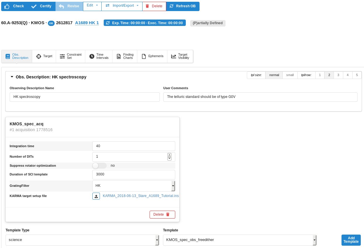
In summary, the set of parameters that you choose in your acquisition template is thus:
- Integration time: 40
- Number of DITs: 1
- Suppress rotator optimization: no
- Duration of SCI template: 3000
- GratingFilter: HK
- KARMA target setup file: KARMA_2013-06-16_Stare_A1689_Tutorial.ins
The acquisition template is now complete, and the window should now look like this:
2.2.3: Target Information
Let us for a moment take a break from inserting templates into this OB.
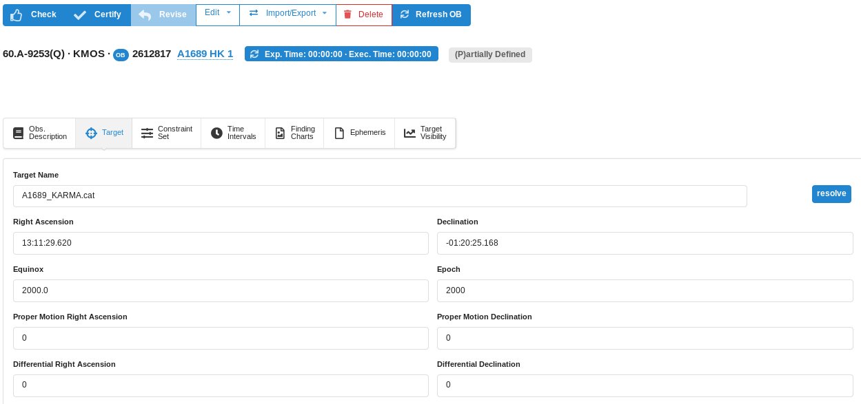
The coordinates (including epoch and equinox) of the science target have been automatically inserted into the Target-tab while uploading the KARMA setup file. Just press the target icon in the icon menu on the top of the OB to have a look. Please never change any of the parameters in this tab!
The values in the target-panel look like this:
2.2.4: Setting the Constraint Set
As stated in Section 1, we assume for the purposes of this tutorial that the program has been allocated time in Service Mode. You thus need to specify a Constraint Set for your OBs. You can do this by clicking on the Constraint Set icon on the top icon menu of the OB and then filling the following entries:
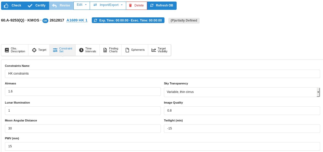
- First, give a descriptive name to the constraint set about to be defined. Since you have decided that this constraint set will be applied to all the OBs, you type 'HK constraints' in the Constraints Name field.
- Since you are not interested in achieving accurate flux calibration of your spectra, you request Variable, thin cirrus conditions in the Sky Transparency entry.
- You would like to spatially resolve your targets. Therefore you should choose a good seeing. Enter 0.8 as value in the Image Quality field.
- Set the Airmass to 1.6, to ensure that your observations are not carried out at too low an elevation.
- Since you are doing spectroscopy in the NIR, the lunar illumination has basically no influence. You should require 1.0 for the Lunar Illumination and 30 degrees for the Moon Angular Distance (smaller values might cause problems linked to the telescope guiding system).
- The Twilight constraint can be relaxed to -15 minutes, since observations in the H- and K-band can be taken without problems before the astronomical twilight ends (negative values).
- Precipitable water vapour (PWV) influences the atmospheric water lines in particular beyond 2 microns. However, for the relative low resolution HK-band telluric lines this does not matter too much. We choose for PWV a value of 15 mm.
Your Constraint Set panel should look like this after entering the values:
Note that in your Phase 1 proposal you already specified some of these constraints (seeing, lunar illumination, transparency). You must make sure that none of the constraints specified in Phase 2 is more stringent than the corresponding one specified at Phase 1.
2.2.5: Setting the time intervals
Since the observations are not time critical we do not have to change anything in the Time Intervals tab. Anyway, clicking on that tab shows the following panel:

With the blue Add button you would be able to define absolute time windows.
2.2.6: Finalising the Observation Description
Target, Constraint Set and Time Intervals are completed, the science template(s) can be inserted.
After checking with the manual and considering the scientific requirements of your program, you have decided to execute the observations using the freedither mode, which allows to freely define the number of dither offsets. The right template is the KMOS_spec_freedither template.
First go back to the Obs. Description button. To select a science template, choose in the Template Type menu on the bottom science. Then select in the Template pull-down menu KMOS_spec_freedither and click on the blue Add Template button next to it. The template appears next to the acquisition template.
Given the flux of your sources and the advice on the duration of the individual DITs in each band as given in the User Manual and checked with the Exposure Time Calculator (ETC), you decide that an appropriate choice of integration time is a DIT of 450 sec. This allows within a 1-hour OB four exposures on target and two exposures on sky. The dither pattern can be, for example: DITHER pattern in ALPHA="0 0.2 0 -0.2" and DITHER pattern in DELTA="0 0 0.2 0". Note that the offsets are defined in an absolute sense, referring to the initial pointing position. I.e. the offsets are not cumulative, relative to the previous position.
For two sky exposures you should set Sky will be observed every X science exposures to 2. This will give a sequence ABA ABA (A=object, B=sky). Since no additional sky exposure is necessary the Exp. time for optional sky can remain zero. Also a repition of the dither pattern is not necessary so you leave the NCYCLES parameter at 1.
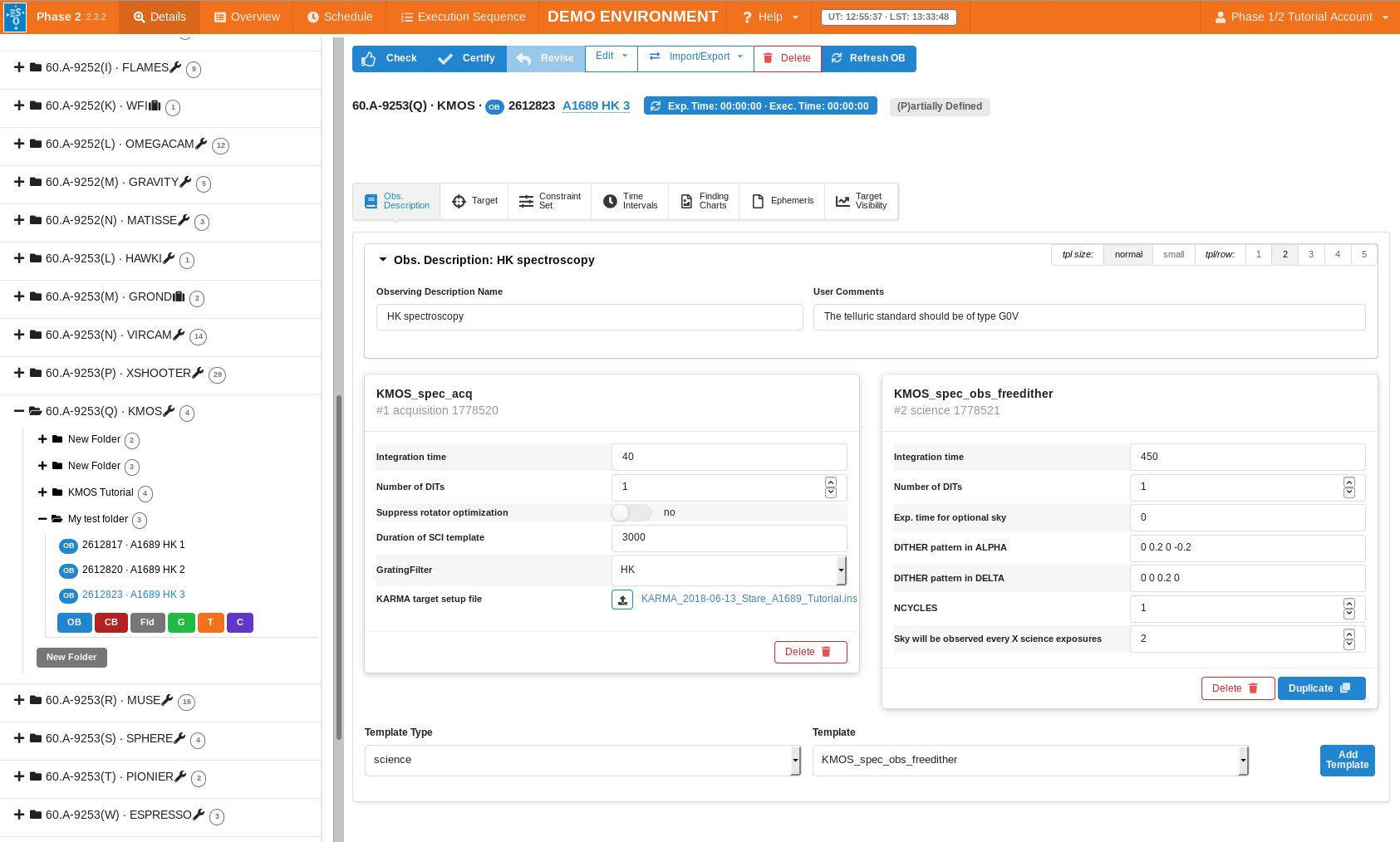
The KMOS_spec_obs_freedither template thus has the following parameters:
- DIT: 450
- NDIT: 1
- Exp. time for optional sky: 0
- DITHER pattern in ALPHA: 0 0.2 0 -0.2
- DITHER pattern in DELTA: 0 0 0.2 0
- NCYCLES: 1
- Sky will be observed every X science exposures: 2
The only other thing that you should really do at this point is to check the execution time for this OB. Press the Exec. Time button on the upper left of top blue menu of the OB. The calculated OB execution time appears in the same button. In this case the total execution time is 01:02:05.0, which is just acceptable for the 1 hour execution time limit.
This completes your first OB! If you followed all the indications given so far, the OB window should look like this now:

Wait! The OB is not entirely complete yet. We have not attached any Finding Charts to the OB yet. Following the general rules and KMOS-specific rules for Finding Chart generation, you make your Finding Chart(s). The jpg file(s) should then be on your local disk, and you attach them to the OB by clicking on the Finding Charts item on the top OB menu, and pressing the blue Upload Finding Chart button. This gives you a browser window, in which you navigate to the correct directory and select the file(s). After the upload your OB window shows a small version of your finding chart, like this one in our case:

Since in this example case, the lensed galaxies around A1689 should be observed for a longer total exposure time to reach the necessary depth, you need to create more OBs, let's say three OBs in total in our case. This can be best done by duplicating the existing OB. Highlight the OB 'A1689 HK 1' in the left menu under your folder, and then press the Edit icon in the top blue menu of the OB, which will give you a pull-down menu with several editing options. Choose the first item Duplicate OB, and this duplicated OB will directly appear in the left menu and the right GUI. You can repeat this procedure to create a second duplication of the original OB. You then can rename the two duplicated OBs as described for the first OB above. In our case the structure of the KMOS run looks then like this:
3: Finishing the preparation and submitting the OBs
Another view of the observing run structure is the Schedule view. In the very top menu click on the tab Schedule. The KMOS runs should then look like this:
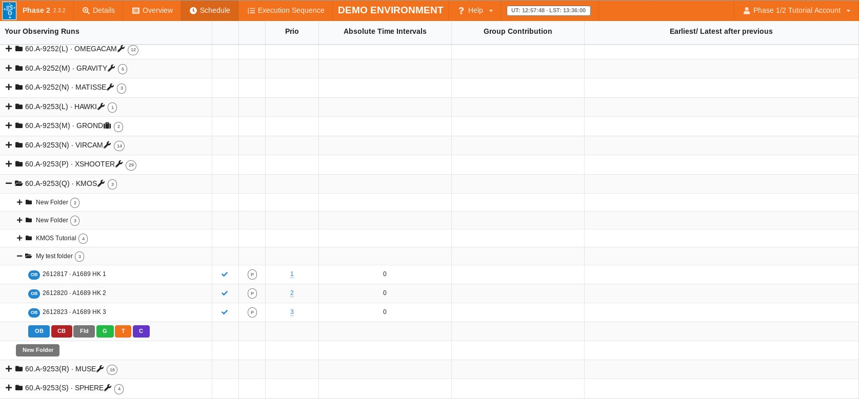
In this view you can assign priorities to the containers or single OBs. You can choose numbers between 1 and 10. The lower the number the higher the priority of the group. In our case, just to illustrate we chose priorities 1, 2 and 3 for the three OBs (although it does not matter for identical OBs which one is observed first).
A general overview of the prepared OBs is given by selecting the Overview button in the very top menu. Our case then looks like this:
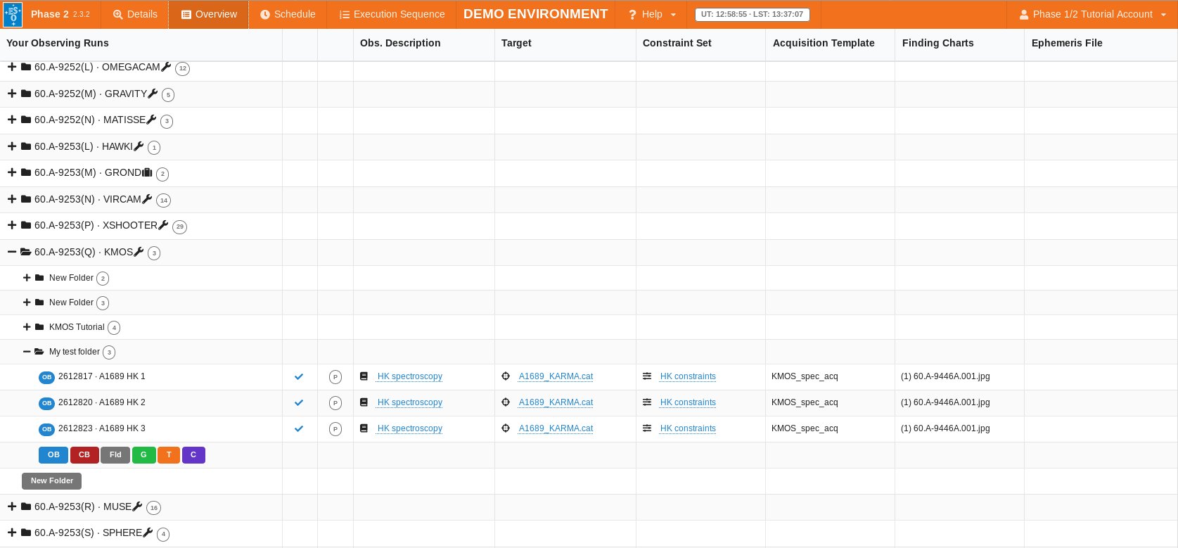
With the completion of the OBs, we consider the example developed in this tutorial to be finished.
However, for a real Service Mode Run, you will have to perform some additional steps. You would also make sure to:
- click the "Check" button (to the right of the Exec. Time button) for each OB. Check performs consistency checks on the selected OB(s).
- click on the Certify" button (to the right of the Check button). Certify does the same as Check, but additionally (if the check was successful) marks the OB(s) as fully compliant and reaxdy for ESO's review. It also marks the OB(s) as readonly.
- (optionally) select one or more certified OBs and click on the "Revise" button (to the right of the Certify button) to revoke the certified status and allow re-editing. If this is done it steps 1 and 2 above should be re-done for the OB(s) in question.
- complete the information in the README file
- click on the "Notify ESO" button (to the right of the Revise button). This will lock all certified OBs as well as the README, in preparation for ESO's Phase 2 review process.
These steps are also explained in more detail on our p2 webpage.
As mentioned above, all users have access to the p2 demo facility. And, unlike the situation that existed with p2's predecessor, P2PP3, all OBs are created directly on the ESO database (there is no longer a "check-in" requirement). Hence, all users can see what you leave behind. Indeed, after a while, if not properly maintained, the p2 demo runs could and would get cluttered with all manner of OBs, containers, etc. Thus, as a courtesy to the next user who follows this tutorial, we would like to ask you to finish these exercises by deleting the OBs, containers, etc. that you make.
Finally, please note that when looking at the tutorial run in the p2 demo facility you will see that both OBs are marked as (+) Accepted. This is a state that these OBs have been set in (by ESO) solely to avoid them being inadvertently deleted from p2.
In another folder 'KMOS Template OBs' you can find some example OBs for the different modes of KMOS (Nod-to-sky, Stare, Freedither, Mosaic24 and Mosaic 8) and standard star observations.