
GRAVITY p2 Tutorial
IMPORTANT: ESO is now offering use of the web application p2 for Phase 2 preparation for all Paranal observing runs from Period 102 onward. The web application p2 fully replaces the use of P2PP for the preparation of the Phase 2 observing material for all telescopes/instruments for both Service and Visitor Mode runs on Paranal. Please check our help section about p2 for instructions on how to notify ESO when your material is ready.
This tutorial provides a step-by-step example of the preparation of a set of OBs with GRAVITY at the ESO-VLTI. The specifics of this tutorial pertain to the preparation of OBs for Period 109 onward.
Please note that all the figures shown below can be clicked on to get higher resolution versions.
To follow this tutorial you should have familiarity with p2, the web-based tool for the preparation of Phase 2 materials, and with the creation of GRAVITY OBs. Please refer to the main p2 webpage (and the items in the menu bar on the left of that page) for a general overview of p2 and generic instructions on the preparation of Observing Blocks (OB). Screenshots for this tutorial were made using the demo mode of p2, but should not differ in any way from one's experience in preparing your own OBs under your run.
The example OBs that we will create in this tutorial are available on the p2 demo version, run 60.A-9252(M) - GRAVITY, in the folder GRAVITY Tutorial.
0: Goal of the Run
In this tutorial we will prepare a snapshot observation of a science target with a dispersed fringe observation in the K-band (2.0-2.4 mu) using GRAVITY's single-field mode and with the high spectral resolution.
VLTI observations generally need to be prepared as concatenations of science (SCI) and calibrator (CAL) OBs. As of P108, such CAL/SCI concatenations can further be organized in groups of concatenations (mandatory for imaging programmes) or time links of concatenations (recommended for time series observations). In this example, we prepare a snapshot observation, which consists simply of a SCI-CAL concatenation.
In case you are interested in using nested containers, that is groups of concatenation (mandatory for imaging) or time links of concatenations, we have prepared a dedicated tutorial on the creation of nested containers for the VLTI.
The example consists of snapshot observation of the Mira variable star S Orionis (Simbad coordinates RA (2000) = 05 29 00.893, Dec (2000) = -04 41 32.75, proper motions RA -11.57 mas/year, Dec -11.34 mas/year) with the short baseline configuration, where the medium baseline configuration can be used an an alternative . We expect an angular uniform disk diameter of 8 mas. Based on the Simbad or 2Mass database, S Ori has an uncorrelated K magnitude of -0.15.
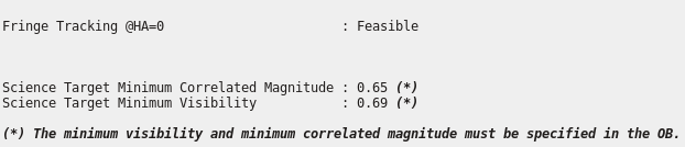
Using this magnitude, the short baseline configuration as primary configuration, and the expected angular diameter, the GRAVITY ETC tells us that the observation is feasible and provides us with the Science Target minumum Correlated Magnitude and the Science Target Minimum Visibility, which we will have to enter below in the Sciene Template. These values correspond to the lowest values of the tracking delay lines:
VLTI OBs are submitted as concatenations of science and calibrator OBs. We will thus also define an OB that describes the observation of a calibrator for S Orionis and we will construct a SCI-CAL concatenation.
These sample OBs in a concatenation will illustrate the use of a variety of features of p2 and the kind of decisions to be taken at the time of preparing in advance an observing run, as well as some aspects that are specific to the preparation of OBs for VLTI and GRAVITY.
1: Getting Started
The Phase 2 process begins when you receive a communication of the ESO Observing Programmes Office (OPO) announcing that the allocation of time for the coming period has been finalized and that you can view the results by logging into the UserPortal and clicking on "Check the webletters."
Let's assume you were granted observing time with GRAVITY in service mode. To start preparing your Phase 2 material including observation blocks, instructions, and finding charts with the web application p2, we recommend you collect all the necessary documentation first:
- The GRAVITY User Manual
- The GRAVITY Template Manual
- The VLTI User Manual
- The VLT Service Mode instructions
- The documentation to the help section about p2 referred to above.
2: Making OBs
2.0: p2
For the sake of this tutorial, we will use the p2 demo facility: https://www.eso.org/p2demo
This is a special facility that ESO has set up so that users who do not have their own p2 login data can still use p2 and prepare example OBs (for example, while writing a proposal to get the overheads right). You cannot use it to prepare actual OBs intended to be executed. When you prepare such OBs you should use your ESO User Portal credentials for p2 (with http://www.eso.org/p2).
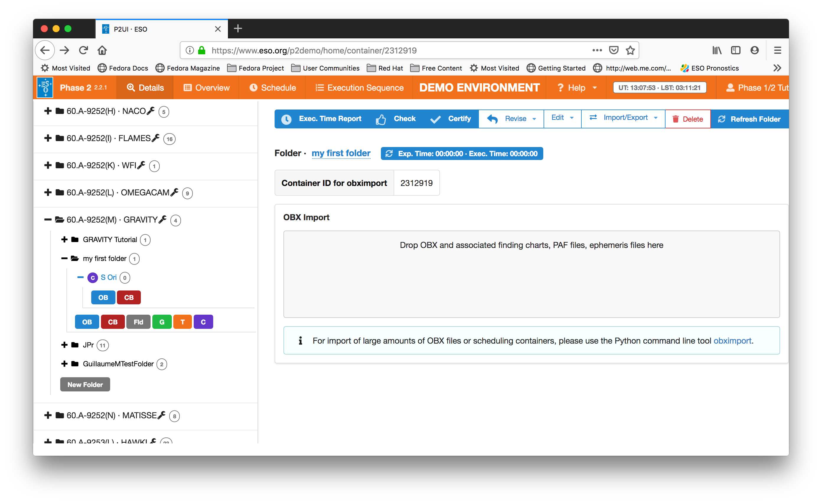
After directing your browser to the p2 demo facility the main p2 GUI will appear as follows: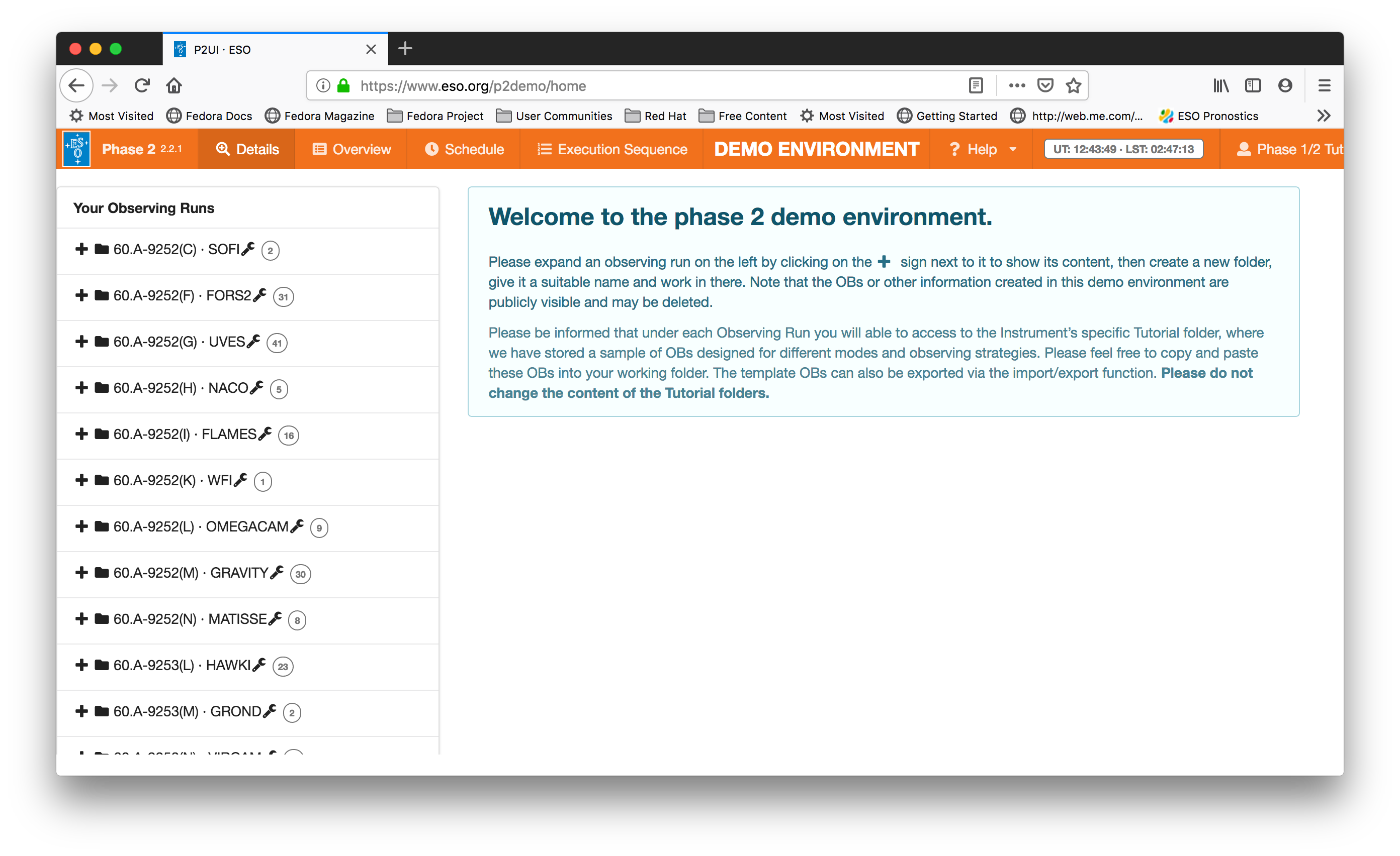
Runs for a number of instruments appear in the lefthand column, since the p2 demo facility is used for all of them. Similarly, if you log into p2 (instead of p2demo) with your own ESO User Portal credentials, you will get the list of all the runs for which you are PI, or for which you have been declared as a Phase 2 delegate by one of your colleagues.
Select the folder corresponding to the GRAVITY tutorial run, 60.A-9252(M) by clicking on the + icon next to it. In this tutorial we assume that time was allocated in Service Mode. This is indicated by the small wrench icon that appears next to the RunID. "Inside the run" you will see (at least) one folder, called "GRAVITY Tutorial". That folder contains the final product of the tutorial you are now reading. You can refer to the contents of that folder at any time, perhaps to compare against your own work. There may be other folders are OBs visible, as this account is a public account and used for testing by other people as well.
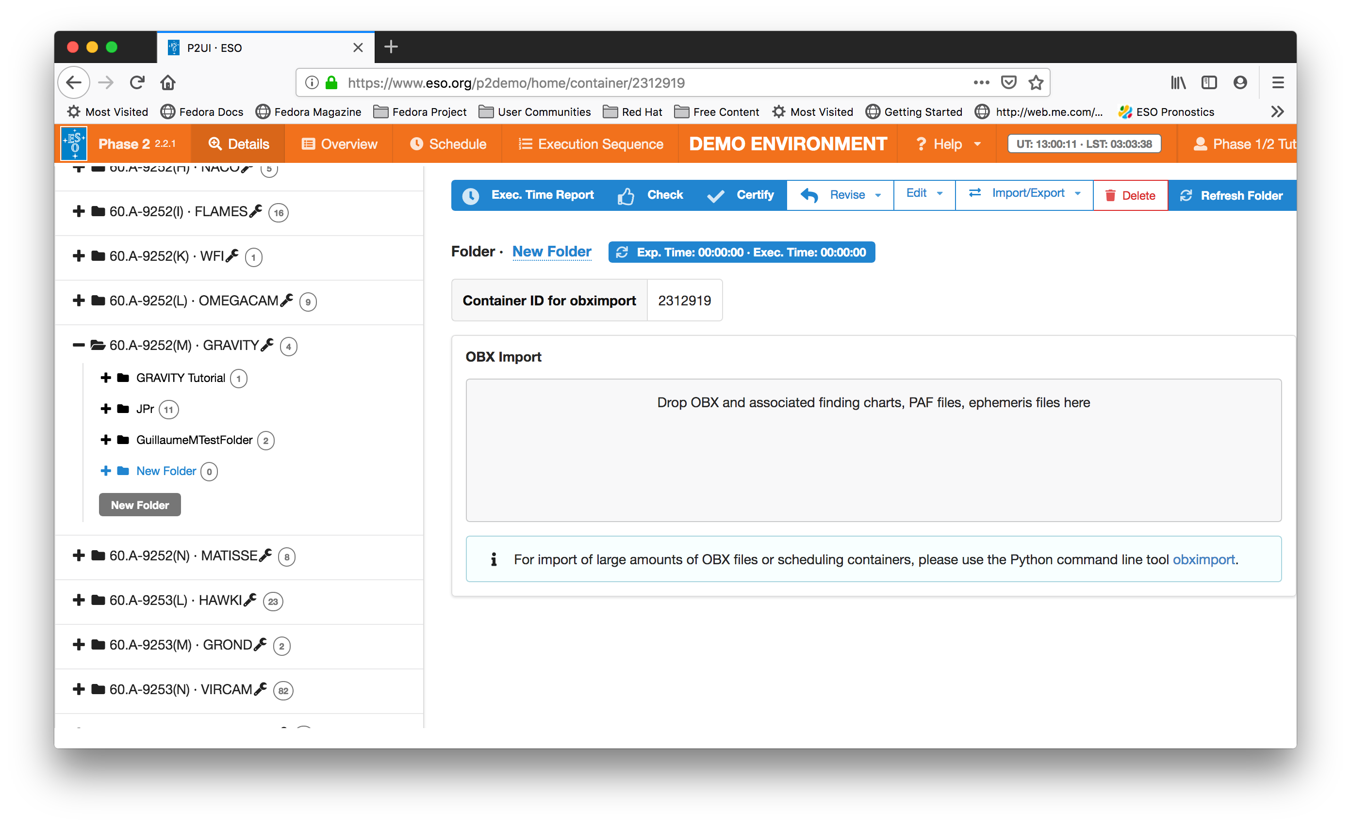
In the p2 demo you must first start by creating a folder, within which you will put your own content.You can create a folder by clicking on the icon New Folder. Please notice that a folder named by default New Folder will appear at the bottom of the list of items in the run. Because the p2 demo is on-line and accessible to anyone you may see folders belonging to other people here, though after-the-fact clean-up is encouraged and possible.
Your screen should look like this after you pressed the "New Folder icon:
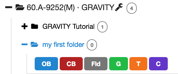
You can give the folder a new name by clicking on the blue 'New folder' text on the top, in this tutorial the name will be "my first folder", but you can set the name of your folder to be (almost) anything you like. Select and open your new folder by clicking on the + icon next to it.
2.1: Creating Containers
Although creating containers is optional in general, all VLTI OBs are normally part of concatenations, which is a type of container in which OBs are executed in sequence. We thus start our tutorial by creating a concatenation container. If you wish to create a standalone OB, please skip this section.
For GRAVITY, the standard sequence is SCI-CAL. Other sequences of science and calibrator OBs may be used as well within the standard limit of uninterrupted service mode observations of 1h (or 1.5h after an approved waiver request). In our example, we wish to define a regular SCI-CAL sequence. We create the concatenation container by clicking on the icon for a concatenation, labeled "C" in purple in the icon bar below your new folder):
This creates an empty container of type concatenation in your folder. Again, as for the folders, type a name for your concatenation container, such as "S Ori". Your window should then look like this:
2.2: Creating OBs
You can now create your first OB within the concatenation container "S Ori": First select your concatenation 'S Ori' in the left menu, then press the blue 'OB'-icon below your (highlighted) concatenation. You will now be able to edit the contents of the OB on the right hand side of the GUI. Enter a name just like you did for the name of the concatenation. The name of the OB must follow the specific OB naming convention for GRAVITY: A science target OB must begin with "SCI_", and a calibrator OB with "CAL_" OB names should also be unique across different runs of the same programme.
We start with creating the science star OB and name it SCI_SOri. Your screen should then look like this:
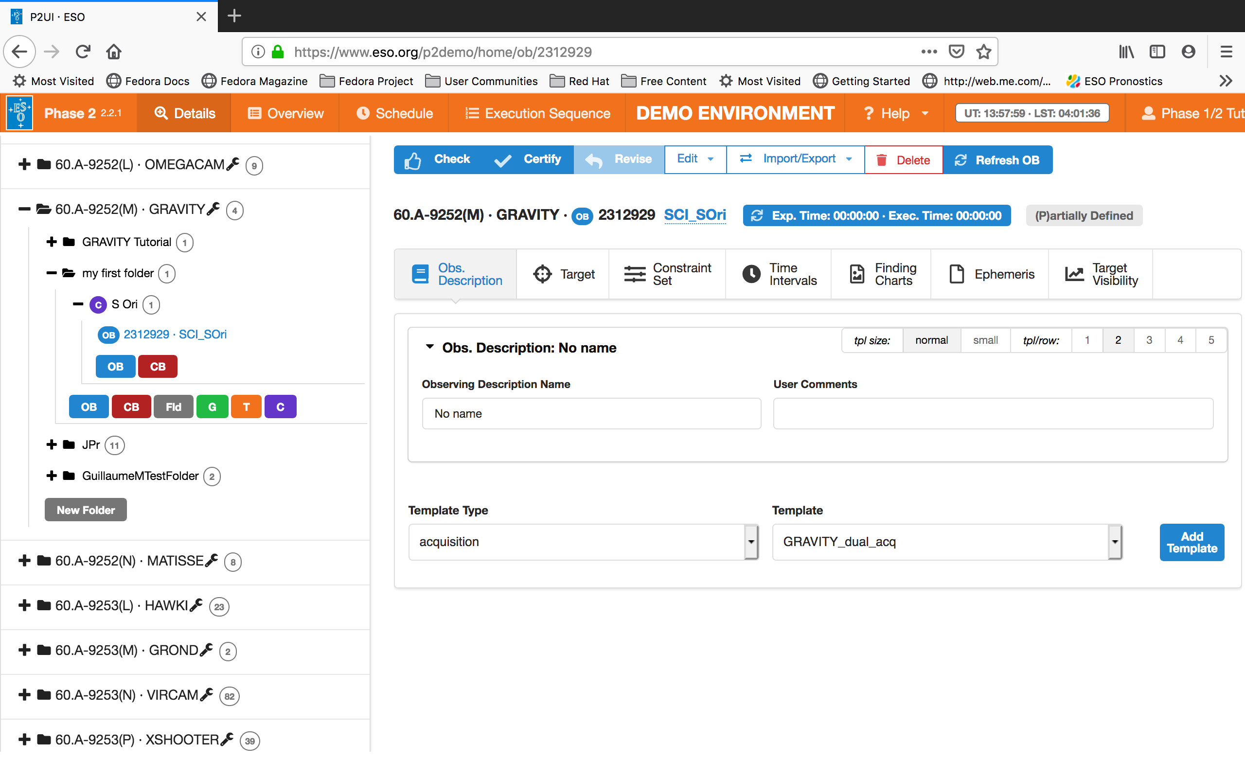
In the next steps, we have to edit the OB information. The relevant fields to be edited are organized within the different tabs below the OB name, called "Obs. Description", "Target", "Constrain Set", "Time Intervals", "Finding Charts" , and "Ephemeris" (relevant for moving targets only). A check of the "Target Visibility" on a certain day is also possible.
2.2.1: Defining the Obs. Description
We start with editing the Obs. Description. This tab is already highlighted in blue in the figure above.
2.2.1.1 Filling in the basic information in the Obs. Description
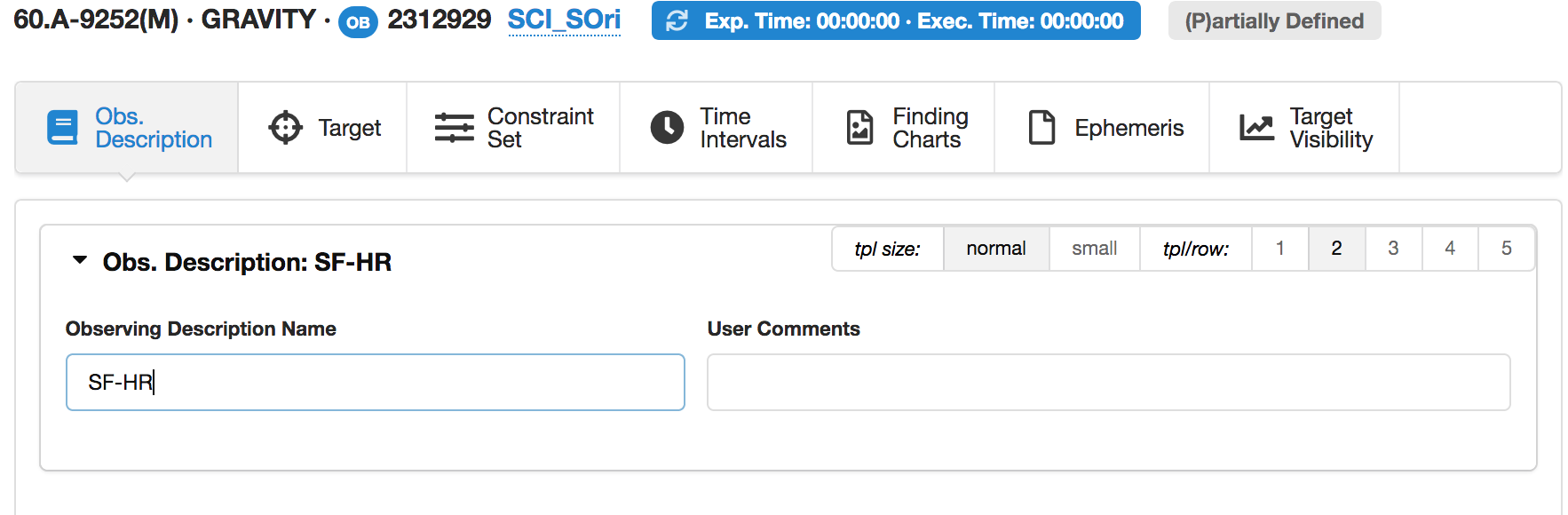
It may be useful in many cases to have an easy way of identifying an observation description, like when having observations of a number of targets performed with identical instrument configuration and exposure times. The Observing Description Name field allows you to fill in an appropriate description. Our example OB is for the single-field mode and the high spectral resolution. We choose "SF-HR".
Next, the User Comments field can be used for any information you wish, e.g. to keep further track of the characteristics of the OB, or to alert the staff on Paranal to special requirements. We do not have any special information for our example OB, so that we leave this field empty.
The top of the OB field should then look like this:
2.2.1.2: Defining the acquisition template
The first template that must be part of any OB is the acquisition template, so let us define it next. In the Template Type list, make sure that the acquisition entry is selected. The Template list on the right contains two acquisition templates available for GRAVITY: GRAVITY_dual_acq and GRAVITY_single_acq, for the GRAVITY dual field and single field modes respectively. Our example is for the single field mode, we thus select GRAVITY_single_acq in the Template list, and press the blue Add Template button next to it:

You need to decide now on the acquisition parameters, which are described in the GRAVITY template manual.
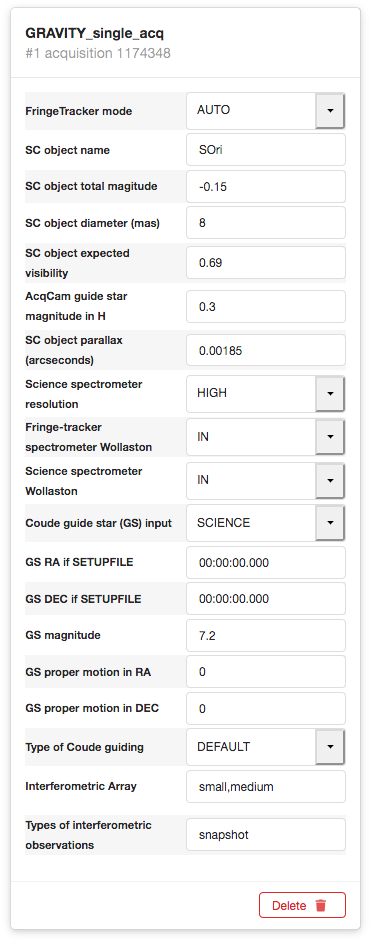
For our observation of S Ori we enter basic information on S Ori and its expected properties, based on the information listed above in the Goal of our example:
- Fringe Tracker mode: AUTO (This is the default mode for the majority of the cases. If object and calibrator have very different magitudes, we might need to force a certain fringe tracker mode as detailed in the template manual)
- SC object name: SOri
- SC object total magnitude: -0.15
- SC object diameter (mas): 8
- SC object expected visibility: 0.69 (from the GRAVITY ETC calculation mentioned above)
- AcqCam guide star magnitude in H: 0.3
- SC object parallax (arcsec): 0.00185
We then set the setup of the GRAVITY instrument according to the example of our science case. We set the instrument setting to high spectral resolution. We decide to put the Wollaston prisms IN, because our target is bright enough. Note that both Wollaston prisms need to be set to the same value:
- Science spectrometer resolution: HIGH
- Fringe-tracker spectrometer Wollaston: IN
- Science-spectometer Wollaston: IN
The next 7 fields correspond to the Coude guide star for STRAP/MACAO. The values for "RA/DEC of guide star if COU guide star is setupfile" are used in cases where the FT target is not bright enough to serve for coude guiding and an off-axis guide star is provided. In that case "COU guide star:SETUPFILE" is chosen. The parameter "GS mag in V" is set to the V magnitude of the target that is used for Coude guiding, whether it is the SC target itself or an off-axis guide star. In our case, S Ori with V=7.2 can serve as a guide star, so that we choose
- Coude guide star (GS) input: SCIENCE
- GS magnitude in V: 7.2
and leave the other GS parameters at their default vaules.
Finally, the last two fields are used to define the baseline configuration and the type of interferometric observation. As we are preparing an OB for the small configuration that could alternatively also be executed with the medium configuration, we add 'small' and 'medium' into 'Interferometric Array', in this order. Our observation is a snapshot observation, so that we add 'snapshot' to 'Types of Interferometric observations":
- Interferometric Array: small, medium
- Types of interferometric observations: snapshot
The acquistion template should then look like this:
2.2.1.3: Defining the science exposure template
In the TemplateType list, select "science". In the case of GRAVITY, "science" refers to recording scientific data on a science target. Since we are preparing an OB for a science target in single field mode, we select the "GRAVITY_single_obs_exp" template and click Add Template. The corresponding templates for calibrator observations are organized under TemplateType "calib". After editing the values the window should now look like this:
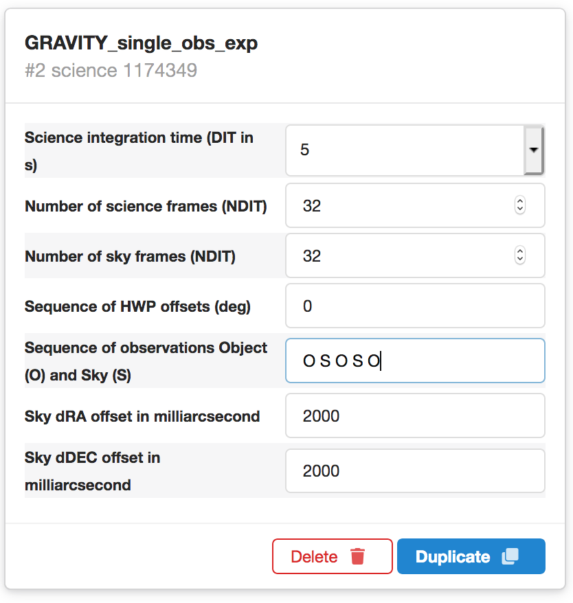
The recommended DIT for our settings is 5 sec according to Table 2 of the GRAVITY template manual (Single-field, HR, Split, AT, K=-0.15). We can well fill our standard allocated time close to 30 minutes per OB by using a OSOSO sequence with NDIT=32. NDIT should be a multiple of 32 or at least of 4. This way, we spend 60% of the time on OBJECT and 40% on SKY, which is a good fraction. We leave the HWP offsets at the standard value of 0. Since our target is a single isolated target, we can leave the sky offsets at their default values.
This completes the filling of the Obs. Description.
2.2.2: Setting the target information
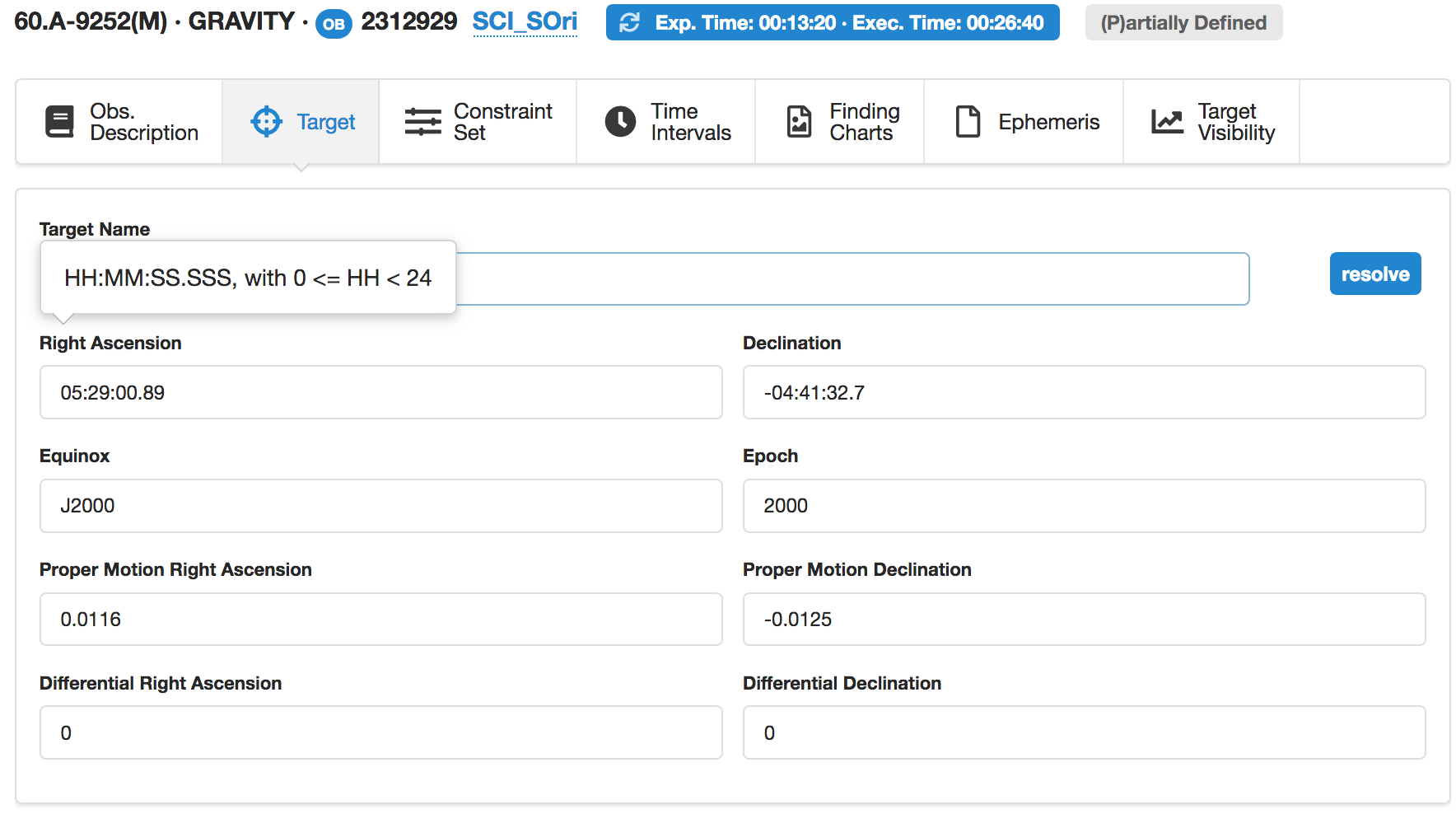
Click on the Target tab at the top of the OB view window in order to insert your target name and coordinates. We should use the same Target Name as used for "SC object name" in the acquisition template. In single field mode, the acqusition target and the science target are the same (for dual field mode, they are different, see the instructions in the template manual for that mode). In the case of VLTI observations, coordinates as precise as possible are essential so that the optical path difference to find the fringes can best be predicted. Therefore, please enter as well the proper motions of the target in arcsec/year (unless not known), preferrably from Gaia DR2 (or newer). The fields Differential RA and Differential Declination are used for differential tracking (solar system objects, for instance), and in our case we leave them with the default values of 0. The acquisition template including the target information is now complete, and the Target view should look like this:
2.2.3: Defining the Constraint Set
As stated in Section 1, we assume for the purposes of this tutorial that the program has been allocated time in Service Mode. You thus need to specify a set of constraints which indicate under which conditions your OB can be executed.You can do this by clicking on the Constraint Set tab on the top of the OB window.
Constraints Name:
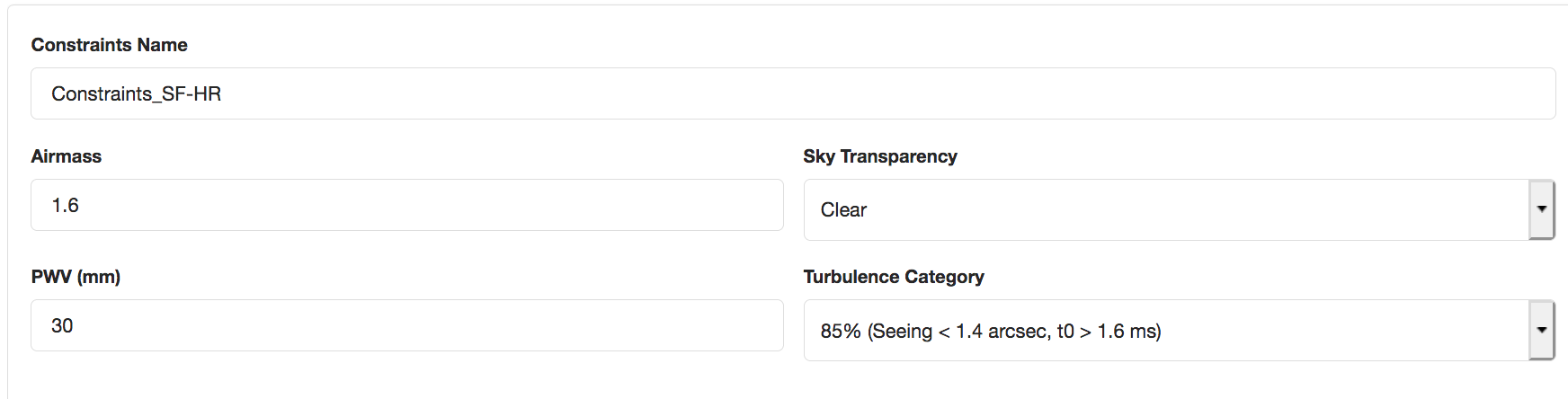
First, give a descriptive name to the constraint set about to be defined. Since you have decided that this constraint set will be applied to all the fringe observations using the single field mode and the high spectral resolution, you type for example "Constraints_SF_HR" in the Constraints Name field.
Note that in your Phase 1 proposal you already specified some of these constraints (sky transparency and seeing) according to the requirements of the GRAVITY instrument webpage. You must make sure that none of the constraints specified in Phase 2 is more stringent than the corresponding ones specified at Phase 1.
Airmass:
The default airmass for GRAVITY observations is 1.6 (corresponding to an altitude above about 40 deg), and should normally not be changed.
Turbulence categoty:
The GRAVITY instrument webpage tells us that a bright target does not need stringent turbulence conditions. We enter the turbulence category T<=85% (seeing<=1.4 arcsec, tau_0>16 ms.
Sky transparency:
The GRAVITY instrument webpage lists the conditions that are required for GRAVITY observations. They generally require that the Sky Transparency condition is "Clear", but that bright stars can also be observed under THIN conditions. We thus choose "Variable, thin cirrus".
PWV:
As for the airmass, the PWV value should be kept at its default, wich is 30 mm.
Your Constraint Set tab should now look like this:
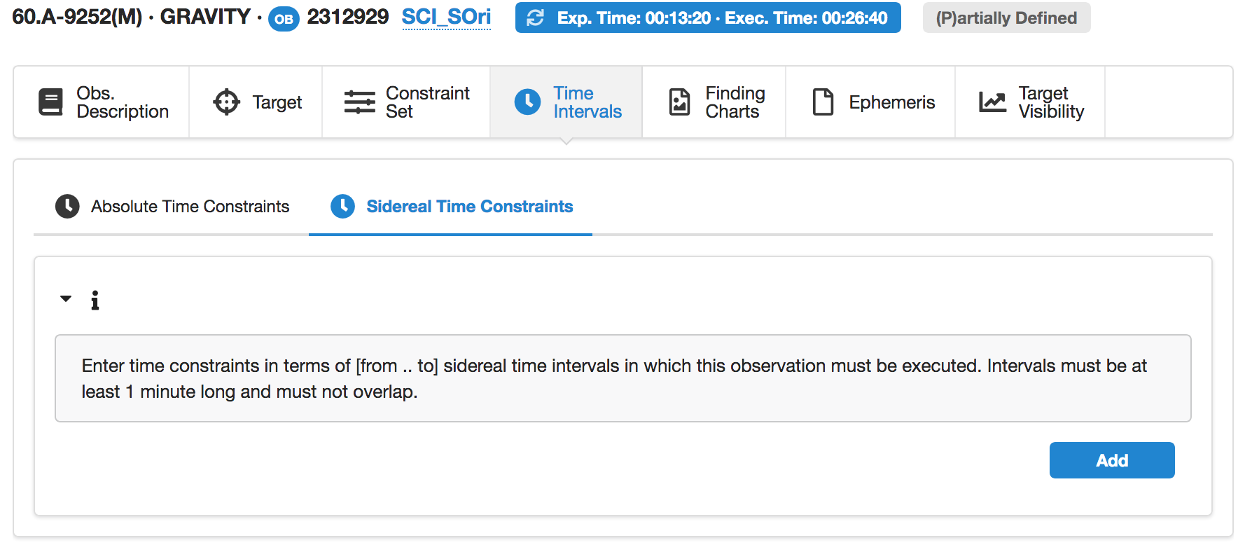
2.2.4: Defining Time Intervals
Click on the Time Intervals tab at the top of the OB window. Here you can specify both Absolute Time Constraints (left tab) and Sidereal Time Constraints (right tab). Both types of time intervals are optional and shall only be used if there is a strong scientific reason to constrain the absolute time or the sidereal time of the observation.
The observability of the target is computed by the observing software on Paranal, so that time intervals shall not be used to purely indicate the observability of the target.
In our case, we do not have a reason to enter either of these time intervals, so that we do not enter anything in this tab.
The "Time Intervals" tab looks like this and we do not change anything:
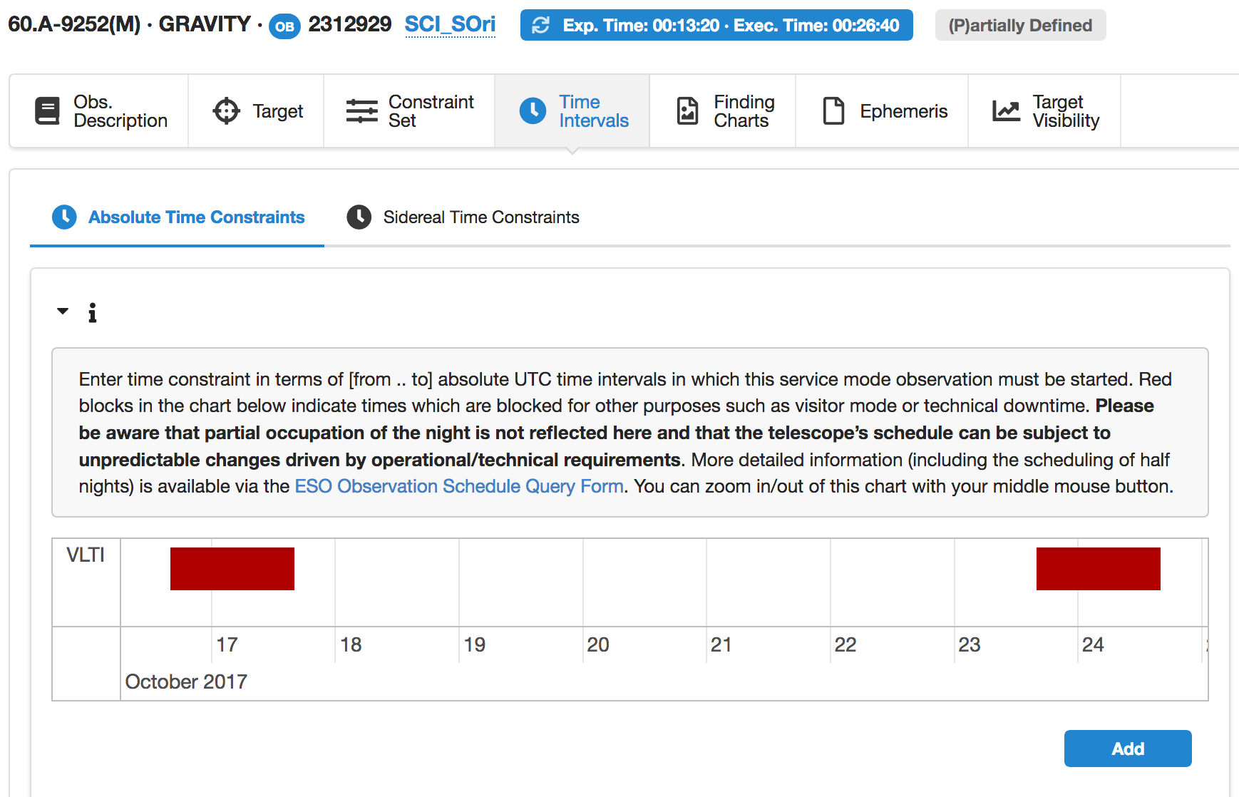
With the blue Add button you would be able to define absolute time windows.
However, we wish to remark that setting time intervals for an OB, and thus narrowing the possible execution time dates, limits the possibility that your OB will be successfully executed during the observing period. Remember that there are only limited service mode time windows over the period, and that any VLTI baseline configuration is scheduled block-wise at certain dates only. It is advisable to double-check the service mode schedule to make sure that the requested baseline configuration is indeed available during your time interval. Your support astronomer will be happy to help you with this.
2.2.4.2: Relative Time Constraints
In principle, p2 allows us to specify relative time links between OBs using time link containers instead of the concatenation container that we used. Indeed, VLTI observations are already required to make use of concatenation containers to specify the sequence of science OBs and calibrator OBs. This means that for VLTI observations the functionality of relative time link containers can not be used (containers of containers are not yet offered). In cases where relative time links between VLTI observations are needed, these should as far as possible be translated into absolute time intervals just as described above, making use of the known block-wise schedule of baseline configurations. Again, your support astronomer will be happy to assist.
2.2.4.3: Sidereal Time Constraints
Sidereal time constraints shall normally not be used, unless there is a strong scientific reason to limit the LST at which the OB shall be excuted. Again, the observability of the OB in terms of altitude, DL limits, shadowing is computed by the observing tool on Paranal, and is not (anymore) encoded into the LST constraint.
We do not enter any Sidereal time constraint, so that the tab looks like this:
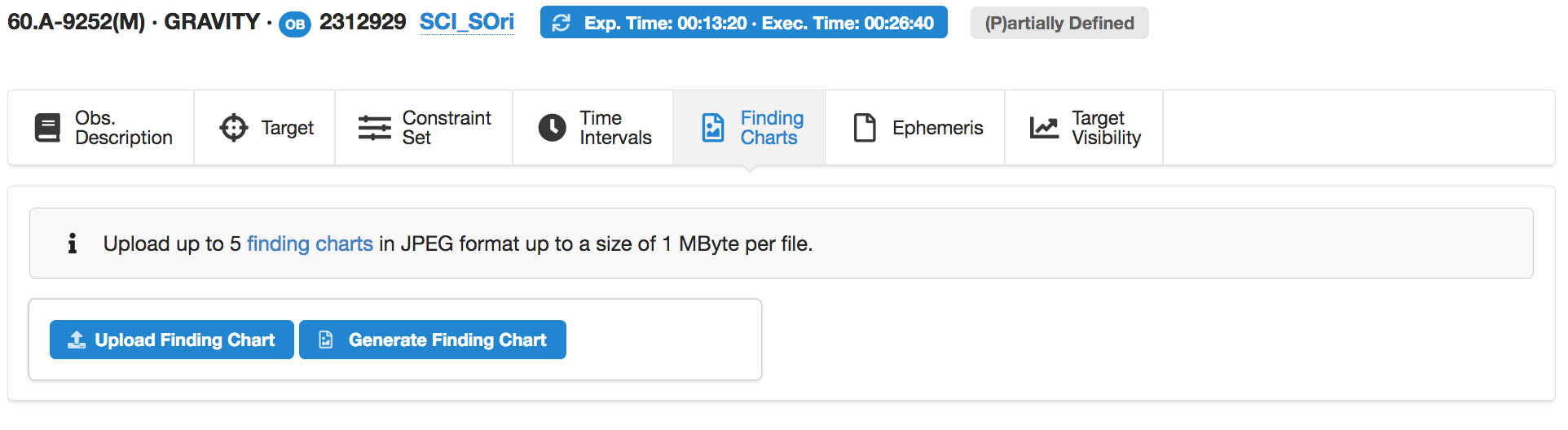
2.2.5: Attaching Finding Charts
The final step of preparing the OB is to attach a Finding Chart. The Finding Charts must be prepared as jpeg-files and must fulfill all general and GRAVITY specific requirements for finding charts. You can use any tool of your choice to create the Finding Charts in jpeg-format. However, the easiest option is to use the tool that is built into p2 to create FCs.
In the 'Finding Charts' tab, you click on "Generate Finding Chart":
This completes the creation of our example OB for S Ori.
2.3: Completing the concatenation and verification
Now, with the first OB of the concatenation completed, you will need to add the calibrator OB next.
To select a calibrator, ESO offers the CalVin tool. CalVin selects suitable calibrators based on different user criteria. Ideally you would wish to have a calibrator star that is unresolved and/or of well known diameter, close on sky to your science target, and of similar brightness. Consulting the CalVin tool you find that the star 31 Ori (HD36167) is a suitable calibrator for your science target S Ori.
The creation of the OB for 31 Ori follows the same procedure as for the science target, except that your OB name is CAL_31Ori and that your fringe recording template is GRAVITY_single_obs_calibrator, which you find for GRAVITY under the calib tab. Of course, you enter the name, the coordinates, and the properties of 31 Ori instead of those of S Ori.
Please make sure that the instrumental settings and baseline configurations are the same for the science target and the calibrator, i.e. we also choose the high spectral resolution, Wollastron prisms IN, and the short baseline configuration as the primary and the medium confguration as alternative choice. Note that, unlike for other VLTI instruments, the DIT does not need to be the same for science target and calibrator. For 31 Ori with its magnitude of K=0.8, the recommended DIT is 5 sec as well, so that we choose DIT=5 sec, NDIT=32, and again a OSOSO sequence.
Before submitting the concatenation to the ESO data base, please check it by first selecting the concatenation S Ori in the menu on the left, and then clicking the Check button (the one with the thumb-up icon). To certify the concatenation, press the Certify button. This will indicate to ESO that the concatenation is ready, and you will not be able to modify it anymore.